mwtoolbox package¶

Submodules¶

mwtoolbox.components module¶

This module involves the calculations related to RF/Microwave components.

mwtoolbox.components.absorptive_filter_equalizer(arg, defaultunits=None)¶

Equalizer using an absorptive filter composed of two coupled lines.

Parameters:

arg (list) –
First 4 arguments are inputs.
1. Reference Impedance ; impedance
2. Coupling (dB) ;
3. Center Frequency ; frequency
4. Test Frequency ; frequency
5. S21 (dB) ;
6. Zeven ; impedance
7. Zodd ; impedance
defaultunits (list, optional) – Default units for quantities in arg list. Default is [] which means SI units will be used if no unit is given in arg.

Returns:

arg

Return type:

list

mwtoolbox.components.awg2dia(arg, defaultunits=None)¶

Convert AWG to Diameter. Reference: Wikipedia, Current rating is calculated through curve fit from online data.

Parameters:

arg (list) –
First 1 arguments are inputs.
1. AWG ;
2. Diameter ;length
3. Current rating in still air ; current
defaultunits (list, optional) – Default units for quantities in arg list. Default is [] which means SI units will be used if no unit is given in arg.

Returns:

arg

Return type:

list

mwtoolbox.components.binomial_quarter_wave_impedance_transformer(arg, defaultunits=None)¶

Binomial Quarter Wave Impedance Transformer.: Reference: Impedance Matching and Transformation.pdf

Parameters:

arg (list) –
First 5 arguments are inputs.
1. Source Impedance;impedance
2. Load Impedance;impedance
3. Number Of Matching Sections;
4. Max(dB(S11)) In Frequency Band ;
5. Center Frequency ; frequency
6. Impedances ; impedance
7. Bandwidth ; frequency
defaultunits (list, optional) – Default units for quantities in arg list. Default is [] which means SI units will be used if no unit is given in arg.

Returns:

arg

Return type:

list

mwtoolbox.components.bridged_tee_attenuator_analysis(arg, defaultunits=None)¶

Bridged Tee Attenuator Analysis.

Parameters:

arg (list) –
First 3 arguments are inputs.
1. Reference Impedance (Zo); impedance
2. Series Impedance (Rs); impedance
3. Parallel Impedance (Rp); impedance
4. S(1,1) ;
5. S(2,1) ;
defaultunits (list, optional) – Default units for quantities in arg list. Default is [] which means SI units will be used if no unit is given in arg.

Returns:

arg

Return type:

list

mwtoolbox.components.bridged_tee_attenuator_synthesis(arg, defaultunits=None)¶

Bridged Tee Attenuator Synthesis.

Parameters:

arg (list) –
First 3 arguments are inputs.
1. Reference Impedance (Zo); impedance
2. Series Impedance (Rs); impedance
3. Parallel Impedance (Rp); impedance
4. S(1,1) ;
5. S(2,1) ;
defaultunits (list, optional) – Default units for quantities in arg list. Default is [] which means SI units will be used if no unit is given in arg.

Returns:

arg

Return type:

list

mwtoolbox.components.chebyshev_quarter_wave_impedance_transformer(arg, defaultunits=None)¶

Chebyshev Quarter Wave Impedance Transformer. Reference: Impedance Matching and Transformation.pdf + eski kod

Parameters:

arg (list) –
First 6 arguments are inputs.
1. Source Impedance ; impedance
2. Load Impedance ; impedance
3. Number Of Matching Sections ;
4. Minimum Frequency ; frequency
5. Maximum Frequency ; frequency
6. Test Frequency ; frequency
7. Impedances ; impedance
8. Return Loss at Test Frequency ;
defaultunits (list, optional) – Default units for quantities in arg list. Default is [] which means SI units will be used if no unit is given in arg.

Returns:

arg

Return type:

list

mwtoolbox.components.chebyshev_taper_impedance_transformer(arg, defaultunits=None)¶

Calculates performance and impedance values for an N-section Chebyshev Impedance Taper. Reference: Foundations for Microwave Engineering, Collin

Parameters:

arg (list) –
First 5 arguments are inputs.
1. Source Impedance ; impedance
2. Load Impedance ; impedance
3. Number Of Sections (Even) ;
4. Fractional Bandwidth (F2/F1) ;
5. Length (normalized to Lambda at fcenter) ;
6. Impedances ; impedance
7. Return Loss ;
defaultunits (list, optional) – Default units for quantities in arg list. Default is [] which means SI units will be used if no unit is given in arg.

Returns:

arg

Return type:

list

mwtoolbox.components.circular_plate_cap(arg, defaultunits=None)¶

Circular Plate Capacitance.

Parameters:

arg (list) –
First 3 arguments are inputs.
1. Radius;length
2. Height;length
3. Dielectric Permittivity;
4. Frequency; frequency
5. Capacitance; capacitance
6. Impedance; impedance
defaultunits (list, optional) – Default units for quantities in arg list. Default is [] which means SI units will be used if no unit is given in arg.

Returns:

arg

Return type:

list

mwtoolbox.components.dia2awg(arg, defaultunits=None)¶

Convert Diameter to AWG. Reference: Wikipedia

Parameters:

arg (list) –
First 1 arguments are inputs.
1. AWG ;
2. Diameter ;length
3. Current rating in still air ; current
defaultunits (list, optional) – Default units for quantities in arg list. Default is [] which means SI units will be used if no unit is given in arg.

Returns:

arg

Return type:

list

mwtoolbox.components.dual_frequency_transformer(arg, defaultunits=None)¶

Dual Frequency Transformer. Reference: A Small Dual Frequency Transformer in Two Sections

Parameters:

arg (list) –
First 4 arguments are inputs.
1. Source Impedance; impedance
2. Load Impedance; impedance
3. f1 Lower Frequency; frequency
4. f2 Higher Frequency; frequency
5. Z1; impedance
6. Z2; impedance
7. Electrical Length ; angle
defaultunits (list, optional) – Default units for quantities in arg list. Default is [] which means SI units will be used if no unit is given in arg.

Returns:

arg

Return type:

list

mwtoolbox.components.dual_transformation1(arg, defaultunits=None)¶

Dual Transformation 1. Reference: Microstrip Filters for RF-Microwave Applications, s.25, Figure 2.6a

Parameters:

arg (list) –
First 4 arguments are inputs.
1. L1 ; inductance
2. C1 ; capacitance
3. L2 ; inductance
4. C2 ; capacitance
5. L1’ ; inductance
6. C1’ ; capacitance
7. L2’ ; inductance
8. C2’ ; capacitance
defaultunits (list, optional) – Default units for quantities in arg list. Default is [] which means SI units will be used if no unit is given in arg.

Returns:

arg

Return type:

list

mwtoolbox.components.dual_transformation2(arg, defaultunits=None)¶

Dual Transformation 1. Reference: Microstrip Filters for RF-Microwave Applications, s.25, Figure 2.6b

Parameters:

arg (list) –
First 4 arguments are inputs.
1. L1 ; inductance
2. C1 ; capacitance
3. L2 ; inductance
4. C2 ; capacitance
5. L1’ ; inductance
6. C1’ ; capacitance
7. L2’ ; inductance
8. C2’ ; capacitance
defaultunits (list, optional) – Default units for quantities in arg list. Default is [] which means SI units will be used if no unit is given in arg.

Returns:

arg

Return type:

list

mwtoolbox.components.evanescent_wg_equivalent(arg, defaultunits=None)¶

Waveguide Width Step from Rectangular Waveguide to Evanescent Mode Rectangular Waveguide. Reference: The Design of Evanescent Mode Waveguide Bandpass Filters for a Prescribed Insertion Loss Characteristic.pdf Model= Xp1,Xs1,Xp1 ya da Xs2,Xp2,Xs2 (p: shunt, s: series) Zo=jXo

Parameters:

arg (list) –
First 5 arguments are inputs.
1. Waveguide Width;length
2. Waveguide Height;length
3. Dielectric Permittivity;
4. Waveguide Length;length
5. Frequency; frequency
6. Series Inductance For Shunt-Series-Shunt Model; inductance
7. Shunt Inductance For Shunt-Series-Shunt Model; inductance
8. Series Inductance For Series-Shunt-Series Model; inductance
9. Shunt Inductance For Series-Shunt-Series Model; inductance
10. Characteristic Impedance; impedance
defaultunits (list, optional) – Default units for quantities in arg list. Default is [] which means SI units will be used if no unit is given in arg.

Returns:

arg

Return type:

list

mwtoolbox.components.ewg_abcd(a, b, er, length, frek)¶

mwtoolbox.components.ewg_inv(a, b, er, length, frek)¶

mwtoolbox.components.exponential_taper_impedance_transformer(arg, defaultunits=None)¶

Exponential Impedance Taper. Reference: Foundations for Microwave Engineering, Collin

Parameters:

arg (list) –
First 5 arguments are inputs.
1. Source Impedance ; impedance
2. Load Impedance ; impedance
3. Number Of Sections ;
4. Fractional Bandwidth (F2/F1) ;
5. Length (normalized to Lambda at fcenter) ;
6. Impedances ; impedance
7. Return Loss ;
defaultunits (list, optional) – Default units for quantities in arg list. Default is [] which means SI units will be used if no unit is given in arg.

Returns:

arg

Return type:

list

mwtoolbox.components.fcutoff_cwg(rad, eps_r=1, v=0, n=1, mode='TE')¶

Computes the cutoff frequency of circular waveguide.

Parameters:

v (int) – Mode number of $\phi$.
n (int) – Radial mode number.
eps_r (float) – Permittivity of filling material.
mode (str) – “TE” or “TM”.
rad (float) – Radius.

Returns:

Cutoff frequency (Hz).

Return type:

fc (float)

mwtoolbox.components.gysel_power_divider(arg, defaultunits=None)¶

Triangle network to Star network transformation. Reference: Zo1: 1. port impedance Zo2: 2. port impedance Zo3: 3. port impedance R1: first isolation resistor (2.porta yakin) R2: second isolation resistor (3.porta yakin) ratio: P2/P3 power ratio Z1: impedance of transmission line between 1.port and 2.port Z2: impedance of transmission line between 1.port and 3.port Z3: impedance of transmission line between 2.port and isolation resistor Z4: impedance of transmission line between 3.port and isolation resistor

Parameters:

arg (list) –
First 6 arguments are inputs.
1. Zo1; impedance
2. Zo2; impedance
3. Zo3; impedance
4. R1; impedance
5. R2; impedance
6. P2/P3 ratio;
7. Z1; impedance
8. Z2; impedance
9. Z3; impedance
10. Z4; impedance
defaultunits (list, optional) – Default units for quantities in arg list. Default is [] which means SI units will be used if no unit is given in arg.

Returns:

arg

Return type:

list

mwtoolbox.components.homogeneous_rect_waveguide_parameters_te(arg, defaultunits=None)¶

Homogeneous Rectangular Waveguide Parameters. Reference: Marcuvitz Waveguide Handbook s.253

Parameters:

arg (list) –
First 10 arguments are inputs.
1. Dielectric Permittivity in Waveguide;
2. Waveguide Width;length
3. Waveguide Height;length
4. Mode (0: Te, 1: Tm);
5. M;
6. N;
7. Tand Of Dielectric;
8. Electrical Conductivity Of Walls; electrical conductivity
9. Frequency; frequency
10. Physical Length;length
11. Cond Loss; loss per length
12. Diel Loss; loss per length
13. Cutoff Freq; frequency
14. Lambda_Guided;length
15. Impedance; impedance
16. Electrical Length; angle
17. Group Velocity;
18. Group Delay; time
defaultunits (list, optional) – Default units for quantities in arg list. Default is [] which means SI units will be used if no unit is given in arg.

Returns:

arg

Return type:

list

mwtoolbox.components.ind_air_core_coil(arg, defaultunits=None)¶

Inductance of a via hole in microstrip. Reference: www.microwavecoil.com , Microwave Components Inc.

Parameters:

arg (list) –
First 4 arguments are inputs.
1. Wire Diameter (d) ;length
2. Coil Inner Diameter (d_in) ;length
3. Spacing Between Turns (s) ; length
4. Number Of Turns ;
5. Inductance ; inductance
6. Resonance Frequency ; frequency
defaultunits (list, optional) – Default units for quantities in arg list. Default is [] which means SI units will be used if no unit is given in arg.

Returns:

arg

Return type:

list

mwtoolbox.components.ind_bond_wire(arg, defaultunits=None)¶

Inductance of a bond wire. Reference: Transmission Line Design Handbook, Wadell, s.153

Parameters:

arg (list) –
First 4 arguments are inputs.
1. Bondwire Radius ;length
2. Substrate Thickness ;length
3. Distance Between End Points ;length
4. Angle At End Points In Degrees ; angle
5. Inductance ;inductance
defaultunits (list, optional) – Default units for quantities in arg list. Default is [] which means SI units will be used if no unit is given in arg.

Returns:

arg

Return type:

list

mwtoolbox.components.ind_microstrip_via_hole(arg, defaultunits=None)¶

Inductance of a via hole in microstrip. Reference: Microstrip Via Hole Grounds in Microstrip.pdf

Parameters:

arg (list) –
First 2 arguments are inputs.
1. Via Radius ;length
2. Substrate Thickness ;length
3. Inductance ; inductance
defaultunits (list, optional) – Default units for quantities in arg list. Default is [] which means SI units will be used if no unit is given in arg.

Returns:

arg

Return type:

list

mwtoolbox.components.ind_straight_flat_wire(arg, defaultunits=None)¶

Inductance of a flat wire. Reference: Transmission Line Design Handbook, Wadell, s.382

Parameters:

arg (list) –
First 6 arguments are inputs.
1. Wire Width ;length
2. Wire Thickness ;length
3. Wire Length ;length
4. Frequency ; frequency
5. Relative Permeability ;
6. Conductivity ; electrical conductivity
7. Inductance ;inductance
8. Impedance ;impedance
defaultunits (list, optional) – Default units for quantities in arg list. Default is [] which means SI units will be used if no unit is given in arg.

Returns:

arg

Return type:

list

mwtoolbox.components.ind_straight_round_wire(arg, defaultunits=None)¶

Inductance of a straight round wire. Reference: Transmission Line Design Handbook, Wadell, s.380

Parameters:

arg (list) –
First 5 arguments are inputs.
1. Wire Diameter ;length
2. Wire Length ;length
3. Frequency ; frequency
4. Dielectric Permeability ;
5. Conductivity ; electrical conductivity
6. Inductance ;inductance
7. Impedance ; impedance
defaultunits (list, optional) – Default units for quantities in arg list. Default is [] which means SI units will be used if no unit is given in arg.

Returns:

arg

Return type:

list

mwtoolbox.components.inductive_post_in_waveguide(arg, defaultunits=None)¶

Inductive Post In Waveguide. Reference: Marcuvitz Waveguide Handbook s.257

Parameters:

arg (list) –
First 6 arguments are inputs.
1. Dielectric Permittivity in Waveguide ;
2. Waveguide Width (a);length
3. Waveguide Height (b);length
4. Post Diameter (d);length
5. Waveguide Sidewall To Post Center (s);length
6. Frequency; frequency
7. Inductance;inductance
8. Capacitance; capacitance
9. Impedance; impedance
defaultunits (list, optional) – Default units for quantities in arg list. Default is [] which means SI units will be used if no unit is given in arg.

Returns:

arg

Return type:

list

mwtoolbox.components.inductive_window_in_waveguide(arg, defaultunits=None)¶

Waveguide Width Step from Rectangular Waveguide to Evanescent Mode Rectangular Waveguide. Reference: Marcuvitz Waveguide Handbook s.253

Parameters:

arg (list) –
First 6 arguments are inputs.
1. Dielectric Permittivity in Waveguide ;
2. Waveguide Width (a);length
3. Waveguide Height (b);length
4. Difference Of Waveguide Width To Window Width;length
5. Window Thickness;length
6. Frequency; frequency
7. Inductance;inductance
8. Capacitance; capacitance
9. Impedance; impedance
defaultunits (list, optional) – Default units for quantities in arg list. Default is [] which means SI units will be used if no unit is given in arg.

Returns:

arg

Return type:

list

mwtoolbox.components.interference_phase_amp_error(arg, defaultunits=None)¶

Maximum phase and amplitude variation of a signal in presence of an interfering signal.

Parameters:

arg (list) –
First 1 arguments are inputs.
1. Difference in dB ;
2. Amplitude Error;
3. Phase Error; angle
defaultunits (list, optional) – Default units for quantities in arg list. Default is [] which means SI units will be used if no unit is given in arg.

Returns:

arg

Return type:

list

mwtoolbox.components.klopfenstein_taper_impedance_transformer(arg, defaultunits=None)¶

Calculates performance and impedance values for an N-section Klopfenstein Impedance Taper. Reference: Microwave Engineering, Pozar

Parameters:

arg (list) –
First 6 arguments are inputs.
1. Source Impedance ; impedance
2. Load Impedance ; impedance
3. Maximum Reflection Coefficient (dB) ;
4. Number Of Sections ;
5. Minimum Frequency ; frequency
6. Test Frequency ; frequency
7. Minimum Total Phase at Minimum Frequency ; angle ;
8. Impedances ; impedance
9. MAG(Reflection Coefficient) ;
defaultunits (list, optional) – Default units for quantities in arg list. Default is [] which means SI units will be used if no unit is given in arg.

Returns:

arg

Return type:

list

mwtoolbox.components.lc_balun(arg, defaultunits=None)¶

Calculate LC Balun.

Parameters:

arg (list) –
First 4 arguments are inputs.
1. Source Impedance (Rin) ; impedance
2. Load Impedances (RL) ; impedance
3. Frequency; frequency
4. Test Frequency ; frequency
5. Inductance ; inductance
6. Capacitance ; capacitance
7. S11 (dB) ;
8. S21 (dB) ;
9. S31 (dB) ;
defaultunits (list, optional) – Default units for quantities in arg list. Default is [] which means SI units will be used if no unit is given in arg.

Returns:

arg

Return type:

list

mwtoolbox.components.optimum_mitered_90_deg_microstrip_bend(arg, defaultunits=None)¶

Optimum Mitered Microstrip Bend Parameters. Reference: Tranmission line design handbook, p.290

Parameters:

arg (list) –
First 2 arguments are inputs.
1. Microstrip Width;length
2. Substrate Height;length
3. Miter Length; length
defaultunits (list, optional) – Default units for quantities in arg list. Default is [] which means SI units will be used if no unit is given in arg.

Returns:

arg

Return type:

list

mwtoolbox.components.optimum_mitered_arbitrary_angle_microstrip_bend(arg, defaultunits=None)¶

Optimum Mitered Microstrip Bend Parameters. Reference: MWOHELP, MBENDA model Burada scipy.interpolate.griddata kullanildi ve maalesef extrapolation yapmiyor. Sinir disi degerlerde dogrudan en yakin deger kullanildi.

Parameters:

arg (list) –
First 2 arguments are inputs.
1. Microstrip Width;length;
2. Substrate Height;length;
3. Angle (0-180 degrees); angle ;
4. Miter Length; length ;
defaultunits (list, optional) – Default units for quantities in arg list. Default is [] which means SI units will be used if no unit is given in arg.

Returns:

arg

Return type:

list

mwtoolbox.components.parallel_plate_cap(arg, defaultunits=None)¶

Parallel Plate Capacitance.

Parameters:

arg (list) –
First 4 arguments are inputs.
1. Width;length
2. Length;length
3. Height;length
4. Dielectric Permittivity;
5. Frequency; frequency
6. Capacitance; capacitance
7. Impedance; impedance
defaultunits (list, optional) – Default units for quantities in arg list. Default is [] which means SI units will be used if no unit is given in arg.

Returns:

arg

Return type:

list

mwtoolbox.components.patch_antenna_analysis(arg, defaultunits=None)¶

Calculates performance and impedance values for an N-section Chebyshev Impedance Taper. Ref: Overview of Microstrip Antennas (Jackson) (Presentation) Reference: Foundations for Microwave Engineering, Collin

Parameters:

arg (list) –
First 6 arguments are inputs.
1. Width (W) ; length
2. Length (L) ; length
3. Substrate Thickness (h);length
4. Dielectric Permittivity ;
5. Dielectric Loss Tangent ;
6. Metal Conductivity ; electrical conductivity
7. Resonance Frequency (f) ; frequency
8. Bandwidth ; frequency
defaultunits (list, optional) – Default units for quantities in arg list. Default is [] which means SI units will be used if no unit is given in arg.

Returns:

arg

Return type:

list

mwtoolbox.components.pcb_track_current_capacity(arg, defaultunits=None)¶

PCB Track Current Capacity.

Parameters:

arg (list) –
First 7 arguments are inputs.
1. Metal Width; length
2. PCB Height; length
3. Metal Thickness; length
4. Allowable Temperature Rise; temperature
5. Thermal Conductivity; thermal conductivity
6. Electrical Conductivity; electrical conductivity
7. External if 1, Internal if 0;
8. Current ; current
defaultunits (list, optional) – Default units for quantities in arg list. Default is [] which means SI units will be used if no unit is given in arg.

Returns:

arg

Return type:

list

mwtoolbox.components.pcb_track_current_capacity_ipc(arg, defaultunits=None)¶

PCB Track Current Capacity, IPC. Reference: IPC2221A

Parameters:

arg (list) –
First 4 arguments are inputs.
1. Metal Width;length
2. Metal Thickness;length
3. Allowable Temperature Rise; temperature
4. External if 1, Internal if 0;
5. Current ; current
defaultunits (list, optional) – Default units for quantities in arg list. Default is [] which means SI units will be used if no unit is given in arg.

Returns:

arg

Return type:

list

mwtoolbox.components.pi_attenuator_analysis(arg, defaultunits=None)¶

Pi Attenuator Analysis.

Parameters:

arg (list) –
First 3 arguments are inputs.
1. Reference Impedance (Zo); impedance
2. Series Impedance (Rs); impedance
3. Parallel Impedance (Rp); impedance
4. S(1,1) ;
5. S(2,1) ;
6. P1 ;
7. P2 ;
8. P3 ;
defaultunits (list, optional) – Default units for quantities in arg list. Default is [] which means SI units will be used if no unit is given in arg.

Returns:

arg

Return type:

list

mwtoolbox.components.pi_attenuator_synthesis(arg, defaultunits=None)¶

Pi Attenuator Analysis.

Parameters:

arg (list) –
First 3 arguments are inputs.
1. Reference Impedance (Zo); impedance
2. Series Impedance (Rs); impedance
3. Parallel Impedance (Rp); impedance
4. S(1,1) ;
5. S(2,1) ;
6. P1 ;
7. P2 ;
8. P3 ;
defaultunits (list, optional) – Default units for quantities in arg list. Default is [] which means SI units will be used if no unit is given in arg.

Returns:

arg

Return type:

list

mwtoolbox.components.rect_wg_to_evanescent_rect_wg_step(a1, a2)¶

Waveguide Width Step from Rectangular Waveguide to Evanescent Mode Rectangular Waveguide. Reference: The Design of Evanescent Mode Waveguide Bandpass Filters for a Prescribed Insertion Loss Characteristic.pdf

Parameters:

arg (list) –
First 2 arguments are inputs.
1. Width of Rectangular Waveguide;length;
2. Width of Evanescent Mode Rectangular Waveguide;length;
3. Inductance; inductance
4. Turns Ratio;
defaultunits (list, optional) – Default units for quantities in arg list. Default is [] which means SI units will be used if no unit is given in arg.

Returns:

arg

Return type:

list

mwtoolbox.components.shorten_90_degree_line(arg, defaultunits=None)¶

Shortening 90 Degree Line with a capacitive load.

Parameters:

arg (list) –
First 3 arguments are inputs.
1. Impedance (Zo); impedance
2. Center Frequency ; frequency
3. Electrical Length (theta) ; angle
4. Impedance (Z); impedance
5. Capacitance ; capacitance
defaultunits (list, optional) – Default units for quantities in arg list. Default is [] which means SI units will be used if no unit is given in arg.

Returns:

arg

Return type:

list

mwtoolbox.components.siw_equivalent_width(w, d, s)¶

Equivalent width of substrate integrated waveguide.

Parameters:

w (float) – Distance between the centers of two via arrays.
d (float) – Diameter of vias.
s (float) – Distance between the centers of consecutive vias of via arrays.

Returns:

Equivalent width of waveguide.

Return type:

float

mwtoolbox.components.star_to_triangle_transformation(arg, defaultunits=None)¶

Star network to Triangle network transformation.: Reference: At star, z1 is connected to A-node, z2 is connected to B-node, z3 is connected to C-node At triangle, z1 is between A-B, z2 is between A-C, z3 is between B-C

Parameters:

arg (list) –
First 3 arguments are inputs.
1. Z1; impedance
2. Z2; impedance
3. Z3; impedance
4. Z1’; impedance
5. Z2’; impedance
6. Z3’; impedance
defaultunits (list, optional) – Default units for quantities in arg list. Default is [] which means SI units will be used if no unit is given in arg.

Returns:

arg

Return type:

list

mwtoolbox.components.symmetric_lange_coupler(arg, defaultunits=None)¶

Symmetric Lange Coupler. Reference: Microwave Circuits, Analysis and Computer-Aided Design, Fusco

Parameters:

arg (list) –
First 3 arguments are inputs.
1. C: Voltage coupling coefficient in dB (positive);
2. n: Number of fingers (should be even);
3. Reference Impedance;impedance
4. Zoo;impedance
5. Zoe;impedance
defaultunits (list, optional) – Default units for quantities in arg list. Default is [] which means SI units will be used if no unit is given in arg.

Returns:

arg

Return type:

list

mwtoolbox.components.tee_attenuator_analysis(arg, defaultunits=None)¶

Tee Attenuator Analysis.

Parameters:

arg (list) –
First 3 arguments are inputs.
1. Reference Impedance (Zo); impedance
2. Series Impedance (Rs); impedance
3. Parallel Impedance (Rp); impedance
4. S(1,1) ;
5. S(2,1) ;
6. P1 ;
7. P2 ;
8. P3 ;
defaultunits (list, optional) – Default units for quantities in arg list. Default is [] which means SI units will be used if no unit is given in arg.

Returns:

arg

Return type:

list

mwtoolbox.components.tee_attenuator_synthesis(arg, defaultunits=None)¶

Tee Attenuator Synthesis.

Parameters:

arg (list) –
First 5 arguments are inputs.
1. Reference Impedance (Zo); impedance
2. Series Impedance (Rs); impedance
3. Parallel Impedance (Rp); impedance
4. S(1,1) ;
5. S(2,1) ;
6. P1 ;
7. P2 ;
8. P3 ;
defaultunits (list, optional) – Default units for quantities in arg list. Default is [] which means SI units will be used if no unit is given in arg.

Returns:

arg

Return type:

list

mwtoolbox.components.thermal_conductance_of_via_farm(arg, defaultunits)¶

Thermal conductance of an array of vias in PCB.

Parameters:

arg (list) –
First 7 arguments are inputs.
1. Plated Via Diameter (d);length
2. Plating Thickness (t);length
3. Area Width (w);length
4. Area Height (l);length
5. Dielectric Height (h);length
6. Number Of Vias (n);
7. Dielectric Thermal Conductivity ; thermal conductivity
8. Metal Thermal Conductivity ; thermal conductivity
9. Thermal Conductance (W/K) ;
10. Thermal Resistance (K/W) ;
defaultunits (list, optional) – Default units for quantities in arg list. Default is [] which means SI units will be used if no unit is given in arg.

Returns:

arg

Return type:

list

mwtoolbox.components.thermal_conductance_of_via_farm_view(arg, defaultunits)¶

mwtoolbox.components.triangle_to_star_transformation(arg, defaultunits=None)¶

Triangle network to Star network transformation. At star, z1 is connected to A-node, z2 is connected to B-node, z3 is connected to C-node At triangle, z1’ is between A-B, z2’ is between A-C, z3’ is between B-C

Parameters:

arg (list) –
Last 3 arguments are inputs.
1. Z1; impedance
2. Z2; impedance
3. Z3; impedance
4. Z1’; impedance
5. Z2’; impedance
6. Z3’; impedance
defaultunits (list, optional) – Default units for quantities in arg list. Default is [] which means SI units will be used if no unit is given in arg.

Returns:

arg

Return type:

list

mwtoolbox.components.triangular_taper_impedance_transformer(arg, defaultunits=None)¶

Triangular Impedance Taper. Reference: Foundations for Microwave Engineering, Collin

Parameters:

arg (list) –
First 5 arguments are inputs.
1. Source Impedance ; impedance
2. Load Impedance ; impedance
3. Number Of Sections (Even) ;
4. Fractional Bandwidth (F2/F1) ;
5. Length (normalized to Lambda at fcenter) ;
6. Impedances ; impedance
7. Return Loss ;
defaultunits (list, optional) – Default units for quantities in arg list. Default is [] which means SI units will be used if no unit is given in arg.

Returns:

arg

Return type:

list

mwtoolbox.components.z_cwg(rad, freq, eps_r=1, v=0, n=1, mode='TE')¶

Computes the wave impedance of circular waveguide.

Parameters:

v (int) – Mode number of $\phi$.
n (int) – Radial mode number.
eps_r (float) – Permittivity of filling material.
freq (float) – Frequency (Hz).
mode (str) – “TE” or “TM”.
rad (float) – Radius.

Returns:

Impedance.

Return type:

Z (float)

mwtoolbox.components.z_wg_te10(er, a, b, freq, formulation=1)¶

mwtoolbox.components.zo_eeff_straight_wire_over_substrate(arg, defaultunits=None)¶

Impedance and Effective Permittivity of Straight Wire Over Substrate. Reference: Transmission Line Design Handbook, Wadell, s.151

Parameters:

arg (list) –
First 4 arguments are inputs.
1. Wire Diameter (d);length
2. Height Of Wire Center Above Ground (h);length
3. Dielectric Thickness (t);length
4. Dielectric Permittivity ;
5. Impedance ; impedance
6. Effective Diel. Permittivity ;
defaultunits (list, optional) – Default units for quantities in arg list. Default is [] which means SI units will be used if no unit is given in arg.

Returns:

arg

Return type:

list

mwtoolbox.components.zo_eeff_wire_on_grounded_substrate(arg, defaultunits=None)¶

Impedance and Effective Permittivity of Straight Wire Over Substrate.: Reference: Transmission Line Design Handbook, Wadell, s.151 Note: eeff is the same as eeff of microstrip with w=2*d, t=0

Parameters:

arg (list) –
First 4 arguments are inputs.
1. Wire Diameter (d);length
2. Dielectric Thickness (t);length
3. Dielectric Permittivity ;
4. Impedance ; impedance
5. Effective Diel. Permittivity ;
defaultunits (list, optional) – Default units for quantities in arg list. Default is [] which means SI units will be used if no unit is given in arg.

Returns:

arg

Return type:

list

mwtoolbox.filters module¶

mwtoolbox.filters.bp_filter_from_prototype(g, Zo, fc, FBW, type=1)¶

mwtoolbox.filters.bs_filter_from_prototype(g, Zo, fc, FBW, type=1)¶

mwtoolbox.filters.butterworth_filter_prototype(n)¶

mwtoolbox.filters.chebyshev_filter_prototype(n, Lar)¶

mwtoolbox.filters.chebyshev_stepped_impedance_lp_filter(Zo, maxreturnloss, N, theta)¶

mwtoolbox.filters.evanescent_wg_filter3(g, n, Lj, a, a1, b, er, fcenter, fbw, alpha)¶

mwtoolbox.filters.evanescent_wg_filter4(g, n, Lj, a, a1, b, er, fcenter, fbw, alpha)¶

mwtoolbox.filters.ewg_abcd(a, b, er, length, frek)¶

mwtoolbox.filters.filter_with_j_inverter(g, Zo, fcenter, fbw, caps)¶

mwtoolbox.filters.filter_with_j_inverter2(g, Zo, fcenter, fbw, caps)¶

mwtoolbox.filters.hp_filter_from_prototype(g, Zo, fc, type=1)¶

mwtoolbox.filters.inductive_post_wg_filter(er, a, b, maxreturnloss, N, d, x, f1, f2)¶

mwtoolbox.filters.lp_filter_from_prototype(g, Zo, fc, type=1)¶

mwtoolbox.filters.minimum_butterworth_filter_degree(L, fstop)¶

mwtoolbox.filters.minimum_chebyshev_filter_degree(Lar, Las, fstop)¶

mwtoolbox.filters.zwg_te10(er, a, b, freq)¶

mwtoolbox.genel module¶

General methods

class mwtoolbox.genel.Flexlist(iterable=(), /)¶

Bases: list

This is a list implementation that supports indexing by list to return some elements of the list

mwtoolbox.genel.annotate_heatmap(im, data=None, valfmt='{x:.2f}', textcolors=('black', 'white'), threshold=None, **textkw)¶

A function to annotate a heatmap. https://matplotlib.org/3.5.0/gallery/images_contours_and_fields/image_annotated_heatmap.html

Parameters:

im – The AxesImage to be labeled.
data – Data used to annotate. If None, the image’s data is used. Optional.
valfmt – The format of the annotations inside the heatmap. This should either use the string format method, e.g. “$ {x:.2f}”, or be a matplotlib.ticker.Formatter. Optional.
textcolors – A pair of colors. The first is used for values below a threshold, the second for those above. Optional.
threshold – Value in data units according to which the colors from textcolors are applied. If None (the default) uses the middle of the colormap as separation. Optional.
kwargs – All other arguments are forwarded to each call to text used to create the text labels.

Usage:: fig, ax = plt.subplots() im, cbar = heatmap(harvest, vegetables, farmers, ax=ax, cmap=”YlGn”, cbarlabel=”harvest [t/year]”) texts = annotate_heatmap(im, valfmt=”{x:.1f} t”)

mwtoolbox.genel.blackman_window(N)¶: Blackman-Harris window Also available in scipy.signal

mwtoolbox.genel.cmp(x, y)¶

Replacement for built-in function cmp that was removed in Python 3

Compare the two objects x and y and return an integer according to the outcome. The return value is negative if x < y, zero if x == y and strictly positive if x > y.

mwtoolbox.genel.coef(birim)¶: SI’dan Birim’e cevirmek icin katsayi

mwtoolbox.genel.convert2pq(sayilar, defaultunits=None)¶: Method to convert a string or string list to float after unit conversion to SI Units are extracted from strings. If there is not a unit in string, unit is taken from defaultunits

mwtoolbox.genel.convert_image(filename, format)¶

mwtoolbox.genel.do_cprofile(func)¶

mwtoolbox.genel.do_profile(follow=[])¶: Helpful if you accidentally leave in production!

class mwtoolbox.genel.dotdict¶

Bases: dict

dot.notation access to dictionary attributes This class is not pickleable!!! objdict is pickleable, because it raises correct exceptions, dill instead of pickle does not work too.

mwtoolbox.genel.ekpolyfit(x)¶: Polynomial fit for ellipk function. works from 0 to 0.98 with good accuracy.

mwtoolbox.genel.flatten(x)¶: Flatten (an irregular) list of lists

mwtoolbox.genel.flatten2(l)¶: Flatten (an irregular) list of lists (yield version of flatten)

mwtoolbox.genel.gaussian_window(sigma, N)¶: Gaussian window sigma should be smaller than or equal to 0.5 Also available in scipy.signal Ref: Wikipedia

mwtoolbox.genel.heatmap(data, row_labels, col_labels, ax=None, cbar_kw={}, cbarlabel='', **kwargs)¶

Create a heatmap from a numpy array and two lists of labels. https://matplotlib.org/3.5.0/gallery/images_contours_and_fields/image_annotated_heatmap.html

Parameters:

data – A 2D numpy array of shape (M, N).
row_labels – A list or array of length M with the labels for the rows.
col_labels – A list or array of length N with the labels for the columns.
ax – A matplotlib.axes.Axes instance to which the heatmap is plotted. If not provided, use current axes or create a new one. Optional.
cbar_kw – A dictionary with arguments to matplotlib.Figure.colorbar. Optional.
cbarlabel – The label for the colorbar. Optional.
kwargs – All other arguments are forwarded to imshow.

Usage:: fig, ax = plt.subplots() im, cbar = heatmap(harvest, vegetables, farmers, ax=ax, cmap=”YlGn”, cbarlabel=”harvest [t/year]”) texts = annotate_heatmap(im, valfmt=”{x:.1f} t”)

class mwtoolbox.genel.objdict¶: Bases: dict

class mwtoolbox.genel.objectview(d)¶: Bases: object

mwtoolbox.genel.peakdet(v, delta, x=None)¶

Converted from MATLAB script at http://billauer.co.il/peakdet.html

Returns two arrays

function [maxtab, mintab]=peakdet(v, delta, x) %PEAKDET Detect peaks in a vector % [MAXTAB, MINTAB] = PEAKDET(V, DELTA) finds the local % maxima and minima (“peaks”) in the vector V. % MAXTAB and MINTAB consists of two columns. Column 1 % contains indices in V, and column 2 the found values. % % With [MAXTAB, MINTAB] = PEAKDET(V, DELTA, X) the indices % in MAXTAB and MINTAB are replaced with the corresponding % X-values. % % A point is considered a maximum peak if it has the maximal % value, and was preceded (to the left) by a value lower by % DELTA.

% Eli Billauer, 3.4.05 (Explicitly not copyrighted). % This function is released to the public domain; Any use is allowed.

mwtoolbox.genel.polarsample(x)¶

Samples the Smith Chart uniformly and returns the reflection coefficient values :param x: Approximate distance between the points. :type x: float

Returns:: list of reflection coefficient values in complex form
Return type:: list

mwtoolbox.genel.prettystring(miktarlar, birim=None)¶

mwtoolbox.genel.printall(isimler, args)¶

mwtoolbox.genel.smooth(x, window_len=11, window='hanning')¶

smooth the data using a window with requested size. This method is based on the convolution of a scaled window with the signal. The signal is prepared by introducing reflected copies of the signal (with the window size) in both ends so that transient parts are minimized in the begining and end part of the output signal.

Parameters:

x (ndarray) – the input signal
window_len (int, optional) – the dimension of the smoothing window; should be an odd integer
window ((string, list, ndarray), optional) –

either
window array with type list or numpy array with size window_len

or
the type of window from ‘flat’, ‘hanning’, ‘hamming’, ‘bartlett’, ‘blackman’

Returns:

the smoothed signal

Example

t=linspace(-2,2,0.1) x=sin(t)+randn(len(t))*0.1 y=smooth(x) see also: numpy.hanning, numpy.hamming, numpy.bartlett, numpy.blackman, numpy.convolve scipy.signal.lfilter

mwtoolbox.genel.split_camel_case(str)¶: Split string written with CamelCase to words. The first letter can be either lower or upper case.

mwtoolbox.genel.str_distance(s, t)¶: levenshtein_ratio_and_distance: Calculates levenshtein distance between two strings. If ratio_calc = True, the function computes the levenshtein distance ratio of similarity between two strings For all i and j, distance[i,j] will contain the Levenshtein distance between the first i characters of s and the first j characters of t

mwtoolbox.genel.stripunit(sayi)¶

mwtoolbox.genel.tukey_window(alpha, N)¶: Tukey window (also known as “tapered cosine window”) Also available in scipy.signal

mwtoolbox.myconstants module¶

mwtoolbox.network module¶

Network Parameters

mwtoolbox.network.abcd2s(M, Zo=50.0)¶: ABCD parameters to S - Parameters conversion. Valid for real Zo value.

mwtoolbox.network.abcd2s_list(M, Zo=50.0)¶: ABCD parameters to S - Parameters conversion. Valid for real Zo value.

mwtoolbox.network.abcd2t(M, Zo=50.0)¶

ABCD parameters to T-Parameters conversion. Valid for real impedances.

ABCD: [V1 I1]=ABCD*[V2 -I2] Pseudo-Wave or Power-Wave? Don’t use for complex impedances.

mwtoolbox.network.abcd2y(M)¶: ABCD parameters to Y-Parameters conversion

mwtoolbox.network.abcd2z(M)¶: ABCD parameters to Z - Parameters conversion

mwtoolbox.network.abcd_change_ports(M)¶: Switching ports of ABCD parameters

mwtoolbox.network.cascade_networks(networks)¶: Cascading 2-port Networks, input and output is ABCD matrices of networks

mwtoolbox.network.circulator()¶: S-parameters of an ideal circulator (circulation direction 1⇒2⇒3)

mwtoolbox.network.connect_2_ports(Smatrix, k, m)¶: Port-m is connected to port-k and both ports are removed Reference: QUCS technical.pdf, S-parameters in CAE programs, p.29

mwtoolbox.network.connect_2_ports_list(Smatrix, conns)¶: Short circuit ports together one-to-one. Short circuited ports are removed. Ports that will be connected are given as tuples in list conn i.e. conn=[(p1,p2),(p3,p4),..] The order of remaining ports is kept. Reference: QUCS technical.pdf, S-parameters in CAE programs, p.29

mwtoolbox.network.connect_2_ports_retain(Smatrix, k, m)¶: Port-m and Port-k are joined to a single port. New port becomes the last port of the circuit. Reference: QUCS technical.pdf, S-parameters in CAE programs, p.29

mwtoolbox.network.connect_network_1_conn(Smatrix, EX, k, m)¶: Port-m of EX circuit is connected to port-k of this circuit Remaining ports of EX are added to the port list of this circuit in order. Reference: QUCS technical.pdf, S-parameters in CAE programs, p.29

mwtoolbox.network.connect_network_1_conn_retain(Smatrix, EX, k, m)¶

mwtoolbox.network.ideal_amp(G)¶: S-parameters of an ideal amplifier/isolator G is voltage gain, no reflection, infinite isolation

mwtoolbox.network.ideal_att(G)¶: S-parameters of an ideal attenuator G is voltage gain (<1), no reflection

mwtoolbox.network.ideal_coupled_line(Ze, Zo, Te, To, Z0)¶: S-parameters of ideal coupled line Te and To in radian 3———-4 1———-2

mwtoolbox.network.ideal_gyrator()¶: S-parameters of ideal gyrator

mwtoolbox.network.ideal_nport(N)¶: S-parameters of ideal N-port junction with equal reference impedances at all ports

mwtoolbox.network.jinv(J)¶: ABCD parameters of J - inverter

mwtoolbox.network.jinv_lumped(X)¶: ABCD parameters of J - inverter produced by 3 inductors in Tee form.

mwtoolbox.network.kinv(K)¶: ABCD parameters of k - inverter

mwtoolbox.network.parallel_networks(networks)¶: Paralleling 2-port Networks, input and output is ABCD matrices of networks

mwtoolbox.network.pi_network(Zp1, Zs, Zp2)¶: ABCD parameters of Pi network

mwtoolbox.network.s2abcd(M, Z=(50.0, 50.0))¶

S-Parameters to ABCD parameters conversion. Valid for real Zo value.

Parameters:: Z (2-tuple, optional) – reference impedance tuple ( Z1, Z2 )

mwtoolbox.network.s2t(M)¶: S-Parameters to Transfer scattering parameters conversion According to definition [b1,a1]=T.[a2,b2] Ref: https://en.wikipedia.org/wiki/Scattering_parameters#Scattering_transfer_parameters

mwtoolbox.network.s2t_list(M)¶: S-Parameters to Transfer scattering parameters conversion According to definition [b1,a1]=T.[a2,b2] Ref: https://en.wikipedia.org/wiki/Scattering_parameters#Scattering_transfer_parameters

mwtoolbox.network.s_normalize_power(S, Zold, Znew)¶: Zold, Znew port_sayisi uzunlugunda dizilerdir Power-Wave icin Reference: Article, “Multiport conversions between S, Z, Y, h, ABCD, and T parameters”

mwtoolbox.network.s_normalize_pseudo(S, Zold, Znew)¶: Zold, Znew port_sayisi uzunlugunda dizilerdir Pseudo-Wave icin

mwtoolbox.network.s_phase_deembed(S, phase)¶: S-parameter deembedding S is numpy.matrix NxN phase, deembedding phase for each port in radian. Positive phase is deembedding into the circuit

mwtoolbox.network.series_networks(networks)¶: Series Connection of Networks (reference pins of 1. network is connected to alive pins of 2. network), input and output is ABCD matrices of networks

mwtoolbox.network.series_z(Z)¶: ABCD parameters of series impedance

mwtoolbox.network.shunt_z(Z)¶: ABCD parameters of shunt impedance

mwtoolbox.network.snp2smp(SM, ports)¶: This method changes the port numbering of the network port j of new network corresponds to ports[j] in old network if the length of “ports” argument is lower than number of ports, remaining ports are terminated with current reference impedances and number of ports are reduced.

mwtoolbox.network.t2abcd(M, Z=(50.0, 50.0))¶: T-parameters to ABCD parameters conversion

mwtoolbox.network.t2s(M)¶: Transfer scattering parameters to S-Parameters conversion According to definition [b1,a1]=T.[a2,b2] Ref: https://en.wikipedia.org/wiki/Scattering_parameters#Scattering_transfer_parameters

mwtoolbox.network.t2s_list(M)¶: Transfer scattering parameters to S-Parameters conversion According to definition [b1,a1]=T.[a2,b2] Ref: https://en.wikipedia.org/wiki/Scattering_parameters#Scattering_transfer_parameters

mwtoolbox.network.t_network(Zs1, Zp, Zs2)¶: ABCD parameters of Tee network

mwtoolbox.network.tline(Zo, theta)¶: ABCD parameters of ideal transmission line, theta = radian

mwtoolbox.network.tline_list(Zo, theta)¶: ABCD parameters of ideal transmission line, theta = radian

mwtoolbox.network.tline_lossy(Zo, gamma)¶: ABCD parameters of lossy transmission line, gamma = complex propagation constant

mwtoolbox.network.transformer(N)¶: ABCD parameters of ideal transformer (1:N)

mwtoolbox.network.y2abcd(M)¶: Y-Parameters to ABCD parameters conversion

mwtoolbox.network.z2abcd(M)¶: Z - Parameters to ABCD parameters conversion

mwtoolbox.networksym module¶

Network Parameters

mwtoolbox.networksym.abcd2s(M, Zo=50)¶: ABCD parameters to S - Parameters conversion Valid for real Zo value

mwtoolbox.networksym.abcd2s_list(M, Zo=50)¶: ABCD parameters to S - Parameters conversion Valid for real Zo value

mwtoolbox.networksym.abcd2t(M, Zo=50)¶

ABCD parameters to T - Parameters conversion

ABCD: [V1 I1]=ABCD*[V2 -I2] Pseudo-Wave or Power-Wave? Don’t use.

mwtoolbox.networksym.abcd2y(M)¶: ABCD parameters to Y - Parameters conversion

mwtoolbox.networksym.abcd2z(M)¶: ABCD parameters to Z - Parameters conversion

mwtoolbox.networksym.abcd_change_ports(M)¶: Switching ports of ABCD parameters

mwtoolbox.networksym.cascade_networks(networks)¶: Cascading 2-port Networks, input and output is ABCD matrices of networks

mwtoolbox.networksym.circulator()¶: S-parameters of an ideal circulator (circulation direction 1⇒2⇒3)

mwtoolbox.networksym.connect_2_ports(Smatrix, k, m)¶: Port-m is connected to port-k and both ports are removed Reference: QUCS technical.pdf, S-parameters in CAE programs, p.29

mwtoolbox.networksym.connect_2_ports_list(Smatrix, conns)¶: Short circuit ports together one-to-one. Short circuited ports are removed. Ports that will be connected are given as tuples in list conn i.e. conn=[(p1,p2),(p3,p4),..] The order of remaining ports is kept. Reference: QUCS technical.pdf, S-parameters in CAE programs, p.29

mwtoolbox.networksym.connect_2_ports_retain(Smatrix, k, m)¶: Port-m and Port-k are joined to a single port. New port becomes the last port of the circuit. Reference: QUCS technical.pdf, S-parameters in CAE programs, p.29

mwtoolbox.networksym.connect_network_1_conn(Smatrix, EX, k, m)¶: Port-m of EX circuit is connected to port-k of this circuit Remaining ports of EX are added to the port list of this circuit in order. Reference: QUCS technical.pdf, S-parameters in CAE programs, p.29

mwtoolbox.networksym.connect_network_1_conn_retain(Smatrix, EX, k, m)¶

mwtoolbox.networksym.ideal_amp(G)¶: S-parameters of an ideal amplifier/isolator G is voltage gain, no reflection, infinite isolation

mwtoolbox.networksym.ideal_att(G)¶: S-parameters of an ideal amplifier/attenuator/isolator G is voltage gain (<1), no reflection

mwtoolbox.networksym.ideal_coupled_line(Ze, Zo, Te, To, Z0)¶: S-parameters of ideal coupled line Te and To in radian 3———-4 1———-2

mwtoolbox.networksym.ideal_gyrator()¶: S-parameters of ideal gyrator

mwtoolbox.networksym.ideal_nport(N)¶: S-parameters of ideal N-port junction with equal reference impedances at all ports

mwtoolbox.networksym.jinv(J)¶: ABCD parameters of J - inverter

mwtoolbox.networksym.jinv_lumped(X)¶: ABCD parameters of J - inverter produced by 3 inductors in Tee form.

mwtoolbox.networksym.kinv(K)¶: ABCD parameters of k - inverter

mwtoolbox.networksym.parallel_networks(networks)¶: Paralleling 2-port Networks, input and output is ABCD matrices of networks

mwtoolbox.networksym.pi_network(Zp1, Zs, Zp2)¶: ABCD parameters of Pi network

mwtoolbox.networksym.s2abcd(M, Z=(50, 50))¶: S-Parameters to ABCD parameters conversion Valid for real Z values Z: reference impedance list [Z1, Z2]

mwtoolbox.networksym.s2t(M)¶: S-Parameters to Transfer scattering parameters conversion According to definition [b1,a1]=T.[a2,b2] Ref: https://en.wikipedia.org/wiki/Scattering_parameters#Scattering_transfer_parameters

mwtoolbox.networksym.s_normalize_power(S, Zold, Znew)¶: Zold, Znew port_sayisi uzunlugunda dizilerdir Power-Wave icin Reference: Article, “Multiport conversions between S, Z, Y, h, ABCD, and T parameters”

mwtoolbox.networksym.s_normalize_pseudo(S, Zold, Znew)¶: Zold, Znew port_sayisi uzunlugunda dizilerdir Pseudo-Wave icin

mwtoolbox.networksym.s_phase_deembed(S, phase)¶: S-parameter deembedding S is sympy.Matrix NxN phase, deembedding phase for each port in radian. Positive phase is deembedding into the circuit

mwtoolbox.networksym.series_networks(networks)¶: Series Connection of Networks (reference pins of 1. network is connected to alive pins of 2. network), input and output is ABCD matrices of networks

mwtoolbox.networksym.series_z(Z)¶: ABCD parameters of series impedance

mwtoolbox.networksym.shunt_z(Z)¶: ABCD parameters of shunt impedance

mwtoolbox.networksym.snp2smp(SM, ports)¶: This method changes the port numbering of the network port j of new network corresponds to ports[j] in old network if the length of “ports” argument is lower than number of ports, remaining ports are terminated with current reference impedances and number of ports are reduced.

mwtoolbox.networksym.t2abcd(M, Z=(50, 50))¶: T-parameters to ABCD parameters conversion

mwtoolbox.networksym.t2s(M)¶: Transfer scattering parameters to S-Parameters conversion According to definition [b1,a1]=T.[a2,b2] Ref: https://en.wikipedia.org/wiki/Scattering_parameters#Scattering_transfer_parameters

mwtoolbox.networksym.t_network(Zs1, Zp, Zs2)¶: ABCD parameters of Tee network

mwtoolbox.networksym.tline(Zo, theta)¶: ABCD parameters of ideal transmission line, theta = radian

mwtoolbox.networksym.tline_list(Zo, theta)¶: ABCD parameters of ideal transmission line, theta = radian

mwtoolbox.networksym.transformer(N)¶: ABCD parameters of ideal transformer (1:N)

mwtoolbox.networksym.y2abcd(M)¶: Y-Parameters to ABCD parameters conversion

mwtoolbox.networksym.z2abcd(M)¶: Z - Parameters to ABCD parameters conversion

mwtoolbox.rfnetwork module¶

mwtoolbox.rfnetwork.average_networks(networks)¶

mwtoolbox.rfnetwork.cascade_2_ports(filenames)¶

mwtoolbox.rfnetwork.extract_gamma_ereff(filename_long_line, filename_short_line, dL, sm=1)¶

Extraction of complex propagation constant (gamma) and complex effective permittivity from the S-Parameters of 2 uniform transmission lines with different lengths.

Parameters:

filename_long_line (str) – S-Parameter filename of longer line.
filename_short_line (str) – S-Parameter filename of shorter line. If None is given, only long line is used for extraction.
dL (float) – Difference of lengths of two lines (positive in meter). If filename_short_line is None, then this is the length of long line.
sm (int, optional) – If this is larger than 1, this is used as number of points for smoothing. Defaults to 1.

Returns:

tuple of two complex numpy arrays (gamma, er_eff).

Return type:

tuple

mwtoolbox.rfnetwork.extract_gamma_ereff_all(files, Ls, sm=1)¶

Extraction of average complex propagation constant (gamma) and complex effective permittivity from the S-Parameters of multiple uniform transmission lines with different lengths.

Parameters:

files (list) – List of S-Parameter filenames of transmission lines.
Ls (list) – List of lengths of transmission lines in the same order as files parameter.
sm (int, optional) – If this is larger than 1, this is used as number of points for smoothing. Defaults to 1.

Returns:

tuple of two complex numpy arrays (gamma, er_eff).

Return type:

tuple

mwtoolbox.rfnetwork.extract_rlgc(spr, length)¶

Extraction of RLGC parameters from S-parameters of a uniform transmission line.

Parameters:

spr (SPFILE) – SPFILE object of two port network.
length (float) – Length of transmission line.

Returns:

tuple of two complex numpy arrays (Inductance per unit length, Characteristic impedance of the line).

Return type:

tuple

mwtoolbox.rfnetwork.generate_multiport_spfile(conf_filename, output_filename)¶

Configuration file format: - comments start by “#” - every line’s format is: “i,j ? filename ? is, js”. The meaning is “S(is,js) of touchstone file filename is S(i,j) of output_filename”

Parameters:

conf_filename (str) – Name of the configuration filename.
output_filename (str) – Name of the output filename.

mwtoolbox.rfnetwork.parse_format(line)¶

class mwtoolbox.rfnetwork.spfile(filename='', freqs=None, n_ports=1, skiplines=0, only_port_number=False)¶

Bases: object

Class that represents an RF network. It can be used to read/write Touchstone files and process RF networks.

file_data_format¶

Format of the data in the file if the data is read from a Touchstone file. Possible values are “DB”, “MA”, “RI”.

Type:: str

file_freq_unit¶

Type:: str

file_name¶

Type:: str

refimpedance¶

Type:: list

sdata¶

Type:: numpy.ndarray

ydata¶

Type:: numpy.ndarray

zdata¶

Type:: numpy.ndarray

abcddata¶

Type:: list

tdata¶

Type:: list

port_names¶

Type:: list

gammas¶

Gamma (propagation constant) values for each port. The shape of the array: (n_ports, frequencypoints). This data is typically read from a touchstone file exported from HFSS.

Type:: numpy.ndarray

inplace¶

Type:: int

s_ok¶

Type:: bool

y_ok¶

Type:: bool

z_ok¶

Type:: bool

t_ok¶

Type:: bool

abcd_ok¶

Type:: bool

sym_smatrix = None

sym_params = dict()

undefinedYindices=set()

undefinedZindices=set()

smatrix_type¶

# 1: “power-wave” # 2: “pseudo-wave” # 3: “HFSS pseudo-wave”

Type:: int

comments¶

# comments in the file before the format line

Type:: list

sparam_gen_func = None # this function generates smatrix of the network given the frequency

sparam_mod_func = None # this function modifies smatrix of the network given the frequency

params¶

Type:: dict

ABCD(i=1, j=1, data_format='COMPLEX', freqs=None)¶

Gives $ABCD_{i j}$ in data_format format. Uses data_array method internally. This is a convenience function for practical use.

Parameters:

i (int, optional) – Port-1. Defaults to 1.
j (int, optional) – Port-2. Defaults to 1.
data_format (str, optional) – See data_format parameter of data_array method. Defaults to “COMPLEX”.
freqs (numpy.ndarray or list, optional) – Frequency points of S-Parameter data. Defaults to None which means data will be calculated for current frequency points of the network.

Returns:

$S_{i j}$ in data_format format

Return type:

numpy.array

Ffunc(imp)¶

Calculates F-matrix in a, b definition of S-Parameters. For internal use of the library.

\[ \begin{align}\begin{aligned}a=F(V+Z_rI)\\b=F(V-Z_r^*I)\end{aligned}\end{align} \]

Parameters:: imp (numpy.ndarray) – Zref, Reference impedance array for which includes the reference impedance for each port.
Returns:: F-Matrix
Return type:: numpy.matrix

S(i=1, j=1, data_format='COMPLEX', freqs=None)¶

Gives $S_{i j}$ in data_format format. Uses data_array method internally. This is a convenience function for practical use.

Parameters:

i (int, optional) – Port-1. Defaults to 1.
j (int, optional) – Port-2. Defaults to 1.
data_format (str, optional) – See data_format parameter of data_array method. Defaults to “COMPLEX”.
freqs (numpy.ndarray or list, optional) – Frequency points of S-Parameter data. Defaults to None which means data will be calculated for current frequency points of the network.

Returns:

$S_{i j}$ in data_format format

Return type:

numpy.array

T(i=1, j=1, data_format='COMPLEX', freqs=None)¶

Return $T_{i j}$ in format data_format Uses data_array method internally. A convenience function for practical use.

Parameters:

i (int, optional) – Port-1. Defaults to 1.
j (int, optional) – Port-2. Defaults to 1.
data_format (str, optional) – See data_format parameter of data_array method. Defaults to “COMPLEX”.

Returns:

$T_{i j}$ as data_format

Return type:

numpy.array

Y(i=1, j=1, data_format='COMPLEX', freqs=None)¶

Return $Y_{i j}$ in format data_format Uses data_array method internally. A convenience function for practical use.

Parameters:

i (int, optional) – Port-1. Defaults to 1.
j (int, optional) – Port-2. Defaults to 1.
data_format (str, optional) – See data_format parameter of data_array method. Defaults to “COMPLEX”.

Returns:

$Y_{i j}$ as data_format

Return type:

numpy.array

Z(i=1, j=1, data_format='COMPLEX', freqs=None)¶

Return $Z_{i j}$ in format data_format Uses data_array method internally. A convenience function for practical use.

Parameters:

i (int, optional) – Port-1. Defaults to 1.
j (int, optional) – Port-2. Defaults to 1.
data_format (str, optional) – See data_format parameter of data_array method. Defaults to “COMPLEX”.

Returns:

$Z_{i j}$ as data_format

Return type:

numpy.array

Z_conjmatch(port1=1, port2=2)¶

Calculates source and load impedances for simultaneous conjugate match.

Parameters:

port1 (int, optional) – [description]. Defaults to 1.
port2 (int, optional) – [description]. Defaults to 2.

Returns:

GS: Reflection coefficient of Port-1 Impedance
GL: Reflection coefficient of Port-2 Impedance

Return type:

2-tuple of numpy.arrays (GS, GL)

__add__(SP2)¶

Implements SP1+SP2. Cascades port-1 of SP2 to port-2 of SP1. Port ordering is shown in the following diagram. Reference impedances of original ports (port-1 of SP1 and port-2 of SP2) are preserved.

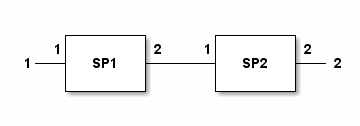
SP1 is self.

Parameters:: SP2 (spfile) – Appended spfile network
Returns:: The result of cascade of 2 networks
Return type:: spfile

__neg__()¶

Calculates an spfile object for two-port networks which is the inverse of this network. This is used to use + and - signs to cascade or deembed 2-port blocks.

Returns:

None if number of ports is not 2.
spfile which is the inverse of the spfile object operated on.

Return type:

spfile

__sub__(SP2)¶

Implements SP1-SP2. Deembeds SP2 from port-2 of SP1. Port ordering is as follows: (1)-SP1-(2)—(1)-SP2-(2) SP1 is self.

Parameters:: SP2 (spfile) – Deembedded spfile network
Returns:: The resulting of deembedding process
Return type:: spfile

add_abs_noise(dbnoise=0.1, phasenoise=0.1, inplace=- 1)¶

This method adds random amplitude and phase noise to the s-parameter data. Mean value for both noises are 0.

Parameters:

dbnoise (float, optional) – Standard deviation of amplitude noise in dB. Defaults to 0.1.
phasenoise (float, optional) – Standard deviation of phase noise in degrees. Defaults to 0.1.
inplace (int, optional) – object editing mode. Defaults to -1.

Returns:

object with noisy data

Return type:

spfile

aliases = {'freqs': 'frequency_points'}¶

calc_syz(input='S', indices=None)¶

This function, using one of S, Y and Z parameters, calculates the other two parameters. Y and Z-matrices calculated separately instead of calculating one and taking inverse. Because one of them may be undefined for some circuits.

Parameters:

input (str, optional) – Input parameter type (should be S, Y or Z). Defaults to “S”.
indices (list, optional) – If given, output matrices are calculated only at the indices given by this list. If it is None, then output matrices are calculated at all frequencies. Defaults to None.

calc_t_eigs(port1=1, port2=2)¶: Eigenfunctions and Eigenvector of T-Matrix is calculated. Only power-wave formulation is implemented.

change_ref_impedance(Znewinput, inplace=- 1)¶

Changes reference impedance and re-calculates S-Parameters.

Parameters:: Znew (float or list) – New Reference Impedance. Its type can be: - float: In this case Znew value is used for all ports - list: In this case each element of this list is assgined to different ports in order as reference impedance. Length of Znew should be equal to number of ports. If an element of the list is None, then the reference impedance for corresponding port is not changed.
Returns:: The spfile object with new reference impedance
Return type:: spfile

change_smatrix_type(smatrix_type)¶

Change S-Matrix formulation and re-calculate s-parameters.

Parameters:: smatrix_type (int) – S-Matrix type. Possible values: 1: Power-Wave, 2:Pseudo-Wave, 3: HFSS Pseudo-Wave

check_passivity()¶

This method determines the frequencies and frequency indices at which the network is not passive. Reference: Fast Passivity Enforcement of S-Parameter Macromodels by Pole Perturbation.pdf For a better discussion: “S-Parameter Quality Metrics (Yuriy Shlepnev)”

Returns:: For non-passive frequencies (indices, frequencies, eigenvalues)
Return type:: 3-tuple of lists

column_of_data(i, j)¶

Gets the indice of column at sdata matrix corresponding to $S_{i j}$ For internal use of the library.

Parameters:

i (int) – First index
j (int) – Second index

Returns:

Index of column

Return type:

int

conj_match_uncoupled(ports=None, inplace=- 1, noofiters=50)¶

Sets the reference impedance for given ports as the complex conjugate of output impedance at each port. The ports are assumed to be uncoupled. Coupling is taken care of by doing the same operation multiple times.

Parameters:

ports (list,optional) – [description]. Defaults to all ports.
inplace (int, optional) – Object editing mode. Defaults to -1.
noofiters (int, optional) – Numberof iterations. Defaults to 50.

Returns:

spfile object with new s-parameters

connect_2_ports(k, m, inplace=- 1)¶

Port-m is connected to port-k and both ports are removed. Reference: QUCS technical.pdf, S-parameters in CAE programs, p.29

Parameters:

k (int) – First port index to be connected.
m (int) – Second port index to be connected.
inplace (int, optional) – Object editing mode. Defaults to -1.

Returns:

New spfile object

Return type:

spfile

connect_2_ports_list(conns, inplace=- 1)¶

Short circuit ports together one-to-one. Short circuited ports are removed. Ports that will be connected are given as tuples in list conns i.e. conns=[(p1,p2),(p3,p4),..] The order of remaining ports is kept. Reference: QUCS technical.pdf, S-parameters in CAE programs, p.29

Parameters:

conns (list of tuples) – A list of 2-tuples of integers showing the ports connected
inplace (int, optional) – Object editing mode. Defaults to -1.

Returns:

New spfile object

Return type:

spfile

connect_2_ports_retain(k, m, inplace=- 1)¶

Port-m is connected to port-k and both ports are removed. New port becomes the last port of the circuit. Reference: QUCS technical.pdf, S-parameters in CAE programs, p.29

Parameters:

k (int) – First port index to be connected.
m (int) – Second port index to be connected.
inplace (int, optional) – Object editing mode. Defaults to -1.

Returns:

New spfile object

Return type:

spfile

connect_network_1_conn(EX, k, m, preserveportnumbers=False, inplace=- 1)¶

Port-m of EX circuit is connected to port-k of this circuit. Both of these ports will be removed. Remaining ports of EX are added to the port list of this circuit in order. Reference: QUCS technical.pdf, S-parameters in CAE programs, p.29

Parameters:

EX (spfile) – External network to be connected to this.
k (int) – Port number of self to be connected.
m (int) – Port number of EX to be connected.
inplace (int, optional) – Object editing mode. Defaults to -1.
preserveportnumbers (bool, optional) – if True, the number of the first added port will be k. Defaults to False.

Returns:

Connected network

Return type:

spfile

connect_network_1_conn_retain(EX, k, m, inplace=- 1)¶

Port-m of EX circuit is connected to port-k of this circuit. This connection point will also be a port. Remaining ports of EX are added to the port list of this circuit in order. The port of connection point will be the last port of the final network. Reference: QUCS technical.pdf, S-parameters in CAE programs, p.29

Parameters:

EX (spfile) – External network to be connected to this.
k (int) – Port number of self to be connected.
m (int) – Port number of EX to be connected.
inplace (int, optional) – Object editing mode. Defaults to -1.
preserveportnumbers1 (bool, optional) – if True, the number of the first added port will be k. Defaults to False.

Returns:

Connected network

Return type:

spfile

convert_s1p_to_s2p()¶

copy()¶

copy_data_from_spfile(local_i, local_j, source_i, source_j, sourcespfile)¶: This method copies S-Parameter data from another SPFILE object

classmethod cpwg_line(length, w, th, er, s, h, freqs=None)¶

Create an spfile object corresponding to a cpwg transmission line.

Parameters:

length (float) – Length of cpwg line.
w (float) – Width of cpwg line.
th (float) – Thickness of metal.
er (float) – Relative permittivity of substrate.
s (float) – Gap of cpwg line.
h (float) – Thickness of substrate.
freqs (float, optional) – Frequency list of object. Defaults to None. If None, frequencies should be set later.

Returns:

An spfile object.

Return type:

spfile

crop_with_frequency(fstart=None, fstop=None, inplace=- 1)¶

Crop the points below fstart and above fstop. No recalculation or interpolation occurs.

Parameters:

fstart (float, optional) – Lower frequency for cropping. Default value is None which means no cropping will occur at lower frequency side.
fstop (float, optional) – Higher frequency for cropping. Default value is None which means no cropping will occur at higher frequency side.
inplace (int, optional) – Object editing mode. Defaults to -1.

Returns:

spfile object with new frequency points.

Return type:

spfile

data_array(data_format='DB', M='S', i=1, j=1, frequencies=None, ref=None, DCInt=0, DCValue=0.0, smoothing=0, InterpolationConstant=0)¶

Return a network parameter between ports i and j ($M_{i j}$) at specified frequencies in specified format.

Parameters:

data_format (str, optional) – Defaults to “DB”. The format of the data returned. Possible values (case insensitive): - “K”: Stability factor of 2-port - “MU1”: Input stability factor of 2-port - “MU2”: Output stability factor of 2-port - “VSWR”: VSWR at port i - “MAG”: Magnitude of $M_{i j}$ - “DB”: Magnitude of $M_{i j}$ in dB - “REAL”: Real part of $M_{i j}$ - “IMAG”: Imaginary part of $M_{i j}$ - “PHASE”: Phase of $M_{i j}$ in degrees between 0-360 - “UPHASE”: Unwrapped Phase of $M_{i j}$ in degrees - “GDELAY”: Group Delay of $M_{i j}$ in seconds
M (str, optional) – Defaults to “S”. Possible values (case insensitive): - “S”: Return S-parameter data - “Y”: Return Y-parameter data - “Z”: Return Z-parameter data - “ABCD”: Return ABCD-parameter data
i (int, optional) – First port number. Defaults to 1.
j (int, optional) – Second port number. Defaults to 1. Ignored for data_format =”VSWR”
frequencies (list, optional) – Defaults to []. List of frequencies in Hz. If an empty list is given, networks whole frequency range is used.
ref (spfile, optional) – Defaults to None. If given the data of this network is subtracted from the same data of ref object.
DCInt (int, optional) – Defaults to 0. If 1, DC point given by DCValue is used at frequency interpolation if frequencies is not [].
DCValue (complex, optional) – Defaults to 0.0. DCValue that can be used for interpolation over frequency.
smoothing (int, optional) – Defaults to 0. if this is higher than 0, it is used as the number of points for smoothing.
InterpolationConstant (int, optional) – Defaults to 0. If this is higher than 0, it is taken as the number of frequencies that will be added between 2 consecutive frequency points. By this way, number of frequencies is increased by interpolation.

Returns:

Network data array

Return type:

numpy.array

extraction(measspfile)¶

Extract die S-Parameters using measurement data and simulated S-Parameters Port ordering in measspfile is assumed to be the same as this spfile. Remaining ports are ports of block to be extracted. See “Extracting multiport S-Parameters of chip” in technical document.

Parameters:: measspfile (spfile) – SPFILE object of measured S-Parameters of first k ports
Returns:: SPFILE object of die’s S-Parameters
Return type:: spfile

gav(port1=1, port2=2, ZS=[], dB=True)¶

Available gain from port1 to port2. If dB=True, output is in dB, otherwise it is a power ratio.

\[G_{av}=\frac{P_{av,toLoad}}{P_{av,fromSource}}\]

Parameters:

port1 (int, optional) – Index of input port. Defaults to 1.
port2 (int, optional) – Index of output port. Defaults to 2.
ZS (list or numpy.ndarray, optional) – Impedance of input port. Defaults to current reference impedance.
dB (bool, optional) – Enable dB output. Defaults to True.

Returns:

Array of Gmax values for all frequencies

Return type:

numpy.ndarray

get_port_number_from_name(isim)¶

Index of first port index with name isim

Parameters:: isim (bool) – Name of the port
Returns:: Port index if port is found, 0 otherwise
Return type:: int

gmax(port1=1, port2=2, dB=True)¶

Calculates Gmax from port1 to port2. Other ports are terminated with current reference impedances. If dB=True, output is in dB, otherwise it is a power ratio.

Parameters:

port1 (int, optional) – Index of input port. Defaults to 1.
port2 (int, optional) – Index of output port. Defaults to 2.
dB (bool, optional) – set True to enable dB output. Defaults to True.

Returns:

Array of Gmax values for all frequencies

Return type:

numpy.ndarray

gop(port1=1, port2=2, ZL=None, dB=True)¶

Operating power gain from port1 to port2 with load impedance of ZL. If dB=True, output is in dB, otherwise it is a power ratio.

\[G_{op}=\frac{P_{toLoad}}{P_{toNetwork}}\]

Parameters:

port1 (int, optional) – Index of input port. Defaults to 1.
port2 (int, optional) – Index of output port. Defaults to 2.
ZL (ndarray or float, optional) – Load impedance. Defaults to current port impedance at port2.
dB (bool, optional) – Enable dB output. Defaults to True.

Returns:

Array of Gop values for all frequencies

Return type:

numpy.ndarray

gop2(port1=1, port2=2, ZL=50.0, dB=True)¶

Operating power gain from port1 to port2 with load impedance of ZL. If dB=True, output is in dB, otherwise it is a power ratio.

\[G_{op}=\frac{P_{toLoad}}{P_{toNetwork}}\]

Parameters:

port1 (int, optional) – Index of input port. Defaults to 1.
port2 (int, optional) – Index of output port. Defaults to 2.
ZL (ndarray or float, optional) – Load impedance. Defaults to current port impedance at port2.
dB (bool, optional) – Enable dB output. Defaults to True.

Returns:

Array of Gop values for all frequencies

Return type:

numpy.ndarray

gt(port1=1, port2=2, ZS=[], ZL=[], dB=True)¶

This method calculates transducer gain (GT) from port1 to port2. Source and load impedances can be specified independently. If any one of them is not specified, current reference impedance is used for that port. Other ports are terminated by reference impedances. This calculation can also be done using impedance renormalization.

\[G_{av}=\frac{P_{load}}{P_{av,fromSource}}\]

Parameters:

port1 (int, optional) – Index of source port. Defaults to 1.
port2 (int, optional) – Index of load port. Defaults to 2.
dB (bool, optional) – Enable dB output. Defaults to True.
ZS (float, optional) – Source impedance. Defaults to 50.0.
ZL (float, optional) – Load impedance. Defaults to 50.0.

Returns:

Array of GT values for all frequencies

Return type:

numpy.ndarray

impulse_response(i=2, j=1, dc_interp=1, dc_value=0.0, max_time_step=1.0, freq_res_coef=1.0, window_name='blackman')¶

Calculates impulse response of $S_{i j}$

Parameters:

i (int, optional) – Port-1. Defaults to 2.
j (int, optional) – Port-2. Defaults to 1.
dc_interp (int, optional) – If 1, add DC point to interpolation. Defaults to 1.
dc_value (float, optional) – dc_value to be used at interpolation if dc_interp=0. Defaults to 0.0. This value is appended to $S_{i j}$ and the rest is left to interpolation in data_array function.
max_time_step (float, optional) – Not used for now. Defaults to 1.0.
freq_res_coef (float, optional) – Coeeficient to increase the frequency resolution by interpolation. Defaults to 1.0 (no interpolation).
window (str, optional) – Windows function to prevent ringing. Defaults to “blackman”. Other windows will be added later.

Returns:

The elements of the tuple are the following in order:

Raw frequency data used as input
Window array
Time array
Time-Domain Waveform of Impulse Response
Time-Domain Waveform of Impulse Input
Time step
Frequency step
Size of input array
Max Value of Impulse Input

Return type:

9-tuple

impulse_response_banded(i=2, j=1, dc_interp=1, dc_value=0.0, max_time_step=1.0, freq_res_coef=1.0, Window='blackman')¶

Calculates impulse response of $S_{i j}$

Parameters:

i (int, optional) – Port-1. Defaults to 2.
j (int, optional) – Port-2. Defaults to 1.
dc_interp (int, optional) – If 1, add DC point to interpolation. Defaults to 1.
dc_value (float, optional) – dc_value to be used at interpolation if dc_interp=0. Defaults to 0.0. This value is appended to $S_{i j}$ and the rest is left to interpolation in data_array function.
max_time_step (float, optional) – Not used for now. Defaults to 1.0.
freq_res_coef (float, optional) – Coeeficient to increase the frequency resolution by interpolation. Defaults to 1.0 (no interpolation).
Window (str, optional) – Windows function to prevent ringing. Defaults to “blackman”. Other windows will be added later.

Returns:

The elements of the tuple are the following in order:

Raw frequency data used as input
Window array
Time array
Time-Domain Waveform of Impulse Response
Time-Domain Waveform of Impulse Input
Time step
Frequency step
Size of input array
Max Value of Impulse Input

Return type:

9-tuple

interpolate(number_of_points=5, inplace=- 1)¶

This method increases the number of frequencies through interpolation.

Parameters:

number_of_points (int, optional) – Number of points used for interpolation. Defaults to 5.
inplace (int, optional) – object editing mode. Defaults to -1.

Returns:

Network object with smooth data

Return type:

spfile

interpolate_data(datain, freqs)¶

Calculate new data corresponding to new frequency points freqs by interpolation from original data corresponding to current frequency points of the network.

Parameters:

data (numpy.ndarray or list) – Original data specified at current frequency points of the network.
freqs (numpy.ndarray or list) – New frequency list.

Returns:

New data corresponding to freqs

Return type:

numpy.ndarray

inverse_2port(inplace=- 1)¶

Take inverse of 2-port data for de-embedding purposes. The reference impedance of the network is not changed.

Parameters:: inplace (int, optional) – Object editing mode. Defaults to -1.
Returns:: Inverted 2-port spfile
Return type:: spfile

load_impedance(Gamma_in, port1=1, port2=2)¶

Calculates termination impedance at port2 that gives Gamma_in reflection coefficient at port1.

Parameters:

Gamma_in (float,ndarray) – Required reflection coefficient.
port1 (int) – Source port.
port2 (int) – Load port.

Returns:

Array of reflection coeeficient of termination at port2

Return type:

numpy.ndarray

make_symmetric(kind=1, inplace=- 1)¶

Make SPFILE symmetric by taking the average of S11 and S22. S12=S21 assumed.

Parameters:: inplace (int, optional) – Object editing mode. Defaults to -1.
Returns:: Modified spfile object
Return type:: spfile

classmethod microstrip_line(length, w, h, t, er, freqs=None)¶

Create an spfile object corresponding to a microstrip line.

Parameters:

length (float) – Length of microstrip line.
w (float) – Width of microstrip line.
h (float) – Thickness of substrate.
t (float) – Thickness of metal.
er (float) – Relative permittivity of microstrip substrate.
freqs (float, optional) – Frequency list of object. Defaults to None. If None, frequencies should be set later.

Returns:

An spfile object.

Return type:

spfile

classmethod microstrip_step(w1, w2, eps_r, h, t, freqs=None)¶

Create an spfile object corresponding to a microstrip step.

Parameters:

w1 (float) – Width of microstrip line at port-1.
w2 (float) – Width of microstrip line at port-2.
t (float) – Thickness of metal.
freqs (float, optional) – Frequency list of object. Defaults to None. If None, frequencies should be set later.

Returns:

An spfile object equivalent to microstrip step.

Return type:

spfile

port_numbers_from_names(*names)¶

This function returns the list of port numbers corresponding to the exact port names given as input parameters.

Parameters:: names (str) – Port names are given as arguments in order.
Returns:: list of port numbers in order.

port_numbers_from_names2(*names)¶

This function returns the list of port numbers corresponding to the port names given as input parameters. For each port name, the port number with closest name is returned. Levenshtein distance is used.

Parameters:: names (str) – Port names are given as arguments in order.
Returns:: list of port numbers in order.

port_numbers_from_names3(*names, cutoff=0.3)¶

This function returns the list of port numbers corresponding to the port names given as input parameters. For each port name, the port number with closest name is returned. Difflib builtin library is used. By default, a cutoff value of 0.3 is used and -1 is returned when no match is found for an input port name.

Parameters:

names (str) – Port names are given as arguments in order.
cutoff (float, optional) – Cutoff value used at difflib library. It should be between 0.0 and 1.0. 1.0 means is perfect match.

Returns:

list of port numbers in order.

prepare_ref_impedance_array(imparray=None)¶

Turns reference impedance array which is composed of numbers,arrays, functions or 1-ports to numerical array which is composed of numbers and arrays. It is made sure that $Re(Z) eq 0$. Mainly for internal use.

Args:
imparray (list, optional): List of impedance array. Default is None.

Returns:
numpy.ndarray: Calculated impedance array

read_file(file_name, skiplines=0, only_port_number=False)¶

Network data is read from file. filename attribute of object is set with given argument.

Parameters:

filename (str) – Name of the file to be read. Its extension should be either “ts” of in the form of “sNp” or “sN”.
skiplines (int, optional) – This option is used if some beginning lines will be ignored. Default value is 0.
only_port_number (bool, optional) – If True, the aim of the file reading is only to get the number of ports and the process is terminated once the port number is determined. Default is False.

read_file_again()¶: Network data is read from the file named filename.

restore_passivity(inplace=- 1)¶

Make the network passive by minimum modification. Reference: Fast and Optimal Algorithms for Enforcing Reciprocity, Passivity and Causality in S-parameters.pdf

Parameters:: inplace (int, optional) – Object editing mode. Defaults to -1.
Returns:: Passive network object
Return type:: spfile

restore_passivity2()¶: Obsolete Bu metod S-parametre datasinin pasif olmadigi frequenciesda S-parametre datasina mumkun olan en kucuk degisikligi yaparak S-parametre datasini pasif hale getirir. Referans: Restoration of Passivity In S-parameter Data of Microwave Measurements.pdf

return_s2p(port1=1, port2=2)¶: Return 2-port s-parameters tuple between port1- and port-2.

s2abcd(port1=1, port2=2)¶

S-Matrix to ABCD matrix conversion between 2 chosen ports. Other ports are terminated with reference impedances

Parameters:

port1 (int, optional) – Index of Port-1. Defaults to 1.
port2 (int, optional) – Index of Port-2. Defaults to 2.

Returns:

ABCD data. Numpy.matrix of size (ns,4) (ns: number of frequencies). Each row contains (A,B,C,D) numbers in order.

Return type:

numpy.matrix

s2t()¶

Calculate transmission matrix for 2-port networks.

Returns:: SPFILE object
Return type:: spfile

scaledata(scale=1.0, dataindices=None)¶: Multiply all elements in S-Parameter matrices by scale.

classmethod series_impedance(Z, freqs=None)¶

Create an spfile object corresponding to a stripline step

Parameters:

R (float) – Shunt resistance.
freqs (float, optional) – Frequency list of object. Defaults to None. If None, frequencies should be set later.

Returns:

An spfile object.

Return type:

spfile

set_data_points(m, indices, x)¶

Set the value for some part of S-Parameter data.

\[S_{i j}[m:m+len(x)]=x\]

Parameters:

m (int) – Starting frequency indice
indices (tuple of int) – Parameters to be set (i,j)
x (number or list) – New value. If this is a number, it is converted to a list.

set_frequencies_wo_recalc(freqs)¶

Directly sets the frequencies of this network, but does not re-calculate s-parameters.

Parameters:: freqs (list or ndarray) – New frequency values

set_frequency_limits(flow, fhigh, inplace=- 1)¶

Remove frequency points higher than fhigh and lower than flow.

Parameters:

flow (float) – Lowest Frequency (Hz)
fhigh (float) – Highest Frequency (Hz)
inplace (int, optional) – Object editing mode. Defaults to -1.

Returns:

spfile object with new frequency points.

Return type:

spfile

set_frequency_points(frequencies, inplace=- 1)¶

Set new frequency points. if S-Parameter data generator function is available, use that to calculate new s-parameter data. If not, use interpolation/extrapolation. For new frequency points, S-Parameters and reference impedances which are in the form of array are re-calculated.

Parameters:

frequencies ((list, numpy.ndarray)) – New frequency array in Hz.
inplace (int, optional) – Object editing mode. Defaults to -1.

Returns:

spfile object with new frequency points.

Return type:

spfile

set_frequency_points_array(fstart, fstop, NumberOfPoints, inplace=- 1)¶

Set the frequencies of the object using start-end frequencies and number of points.

Parameters:

fstart ([type]) – Start frequency.
fstop ([type]) – End frequency.
NumberOfPoints (int) – Number of frequencies.
inplace (int, optional) – Object editing mode. Defaults to -1.

Returns:

spfile object with new frequency points.

Return type:

spfile

set_port_name(name, i)¶

Set name of a specific port.

Parameters:

name (str) – New name of the port
i (int) – Port number

set_smatrix_at_frequency_point(indices, smatrix)¶

Set S-Matrix at frequency indices

Parameters:

indices (list) – List of frequency indices
smatrix (numpy.matrix) – New S-Matrix value which is to be set at all indices

set_smatrix_type(smatrix_type)¶

set_sparam_gen_func(func=None)¶

This function is used to set the function that generates s-parameters from frequency.

Parameters:: func (function, optional) – function to be set. Defaults to None.

set_sparam_mod_func(func=None)¶

This function is used to set the function that generates s-parameters from frequency.

Parameters:: func (function, optional) – function to be set. Defaults to None.

set_sym_params(paramdict)¶

This function is used to set the values of symbolic variables of the network. This is used if the S-Matrix of the network is defined by an arithmetic expression containing symbolic variables. This property is used in conjunction with sympy library for symbolic manipulation. Arithmetic expression for S-Matrix is defined by set_sym_smatrix function.

Parameters:: paramdict (dict) – This is a dictionary containing the values of symbolic variables of the network

set_sym_smatrix(SM)¶

This function is used to set arithmetic expression for S-Matrix, if S-Matrix is defined using symbolic variables.

Parameters:: SM (sympy.Matrix) – Symbolic sympy.Matrix expression for S-Parameter matrix

classmethod shunt_impedance(Z, freqs=None)¶

Create an spfile object corresponding to a stripline step

Parameters:

R (float) – Shunt resistance.
freqs (float, optional) – Frequency list of object. Defaults to None. If None, frequencies should be set later.

Returns:

An spfile object.

Return type:

spfile

smoothing(smoothing_length=5, inplace=- 1)¶

This method applies moving average smoothing to the s-parameter data

Parameters:

smoothing_length (int, optional) – Number of points used for smoothing. Defaults to 5.
inplace (int, optional) – object editing mode. Defaults to -1.

Returns:

Network object with smooth data

Return type:

spfile

snp2smp(ports, inplace=- 1)¶

This method changes the port numbering of the network port j of new network corresponds to ports[j] in old network.

if the length of “ports” argument is lower than number of ports, remaining ports are terminated with current reference impedances and number of ports are reduced.

Parameters:

ports (list) – New port order
inplace (int, optional) – Object editing mode. Defaults to -1.

Returns:

Modified spfile object

Return type:

spfile

sqrt_network()¶

Calculate the spfile, when two of which are cascaded, this spfile is obtained.

Returns:: SPFILE object
Return type:: spfile

stability_factor_k(port1=1, port2=2)¶

Calculates k stability factor, from port1 to port2. Other ports are terminated with reference impedances.

Parameters:

port1 (int, optional) – Index of source port. Defaults to 1.
port2 (int, optional) – Index of load port. Defaults to 2.

Returns:

Array of stability factor for all frequencies

Return type:

numpy.ndarray

stability_factor_mu1(port1=1, port2=2)¶

Calculates $\mu_1$ stability factor, from port1 to port2. Other ports are terminated with reference impedances.

Parameters:

port1 (int, optional) – Index of source port. Defaults to 1.
port2 (int, optional) – Index of load port. Defaults to 2.

Returns:

Array of stability factor for all frequencies

Return type:

numpy.ndarray

stability_factor_mu2(port1=1, port2=2)¶

Calculates $\mu_2$ stability factor, from port1 to port2. Other ports are terminated with reference impedances.

Parameters:

port1 (int, optional) – Index of source port. Defaults to 1.
port2 (int, optional) – Index of load port. Defaults to 2.

Returns:

Array of stability factor for all frequencies

Return type:

numpy.ndarray

classmethod stripline(length, w, er, h1, h2, t, freqs=None)¶

Create an spfile object corresponding to a stripline transmission line.

Parameters:

length (float) – Length of cpwg line.
w (float) – Width of stripline.
er (float) – Relative permittivity of substrate.
h1 (float) – Thickness of substrate from bottom ground to bottom of line.
h2 (float) – Thickness of substrate from top line to top ground.
t (float) – Thickness of metal.
freqs (float, optional) – Frequency list of object. Defaults to None. If None, frequencies should be set later.

Returns:

An spfile object.

Return type:

spfile

classmethod stripline_step(w1, w2, eps_r, h1, h2, t, freqs=None)¶

Create an spfile object corresponding to a stripline step

Parameters:

w1 (float) – Width of stripline line at port-1.
w2 (float) – Width of stripline line at port-2.
eps_r (float) – Relative permittivity of stripline substrate.
h (float) – Thickness of stripline substrate.
t (float) – Thickness of metal.
freqs (float, optional) – Frequency list of object. Defaults to None. If None, frequencies should be set later.

Returns:

An spfile object.

Return type:

spfile

uniform_deembed(quantity, ports='all', kind='degrees', inplace=- 1)¶

This function deembeds some of the ports of S-Parameters. Deembedding quantity can be:

Phase in degrees
Phase in radians
Length in meters
Delay in seconds

A positive quantity means deembedding into the circuit. The Zc of de-embedding lines is the reference impedances of each port.

Parameters:

quantity (float or list) – Quantity to be deembedded. - If a number is given, it is used for all frequencies and ports - If a list is given, if its size is 1, its element is used for all ports. If its size is equal to number of ports, the list is used for all frequencies. If size>1, then size should be equal to the number of frequencies. If an element of list is number, it is used for all ports. If an element of the list is also a list, the elements size should be same as the number of ports.
ports (list, optional) – List of port numbers to be deembedded. If not given all ports are deembedded.
kind (string, optional) – One of the following values, “degrees”, “radians”, “length” and “delay”. Defaults to “degrees”.
inplace (int, optional) – Object editing mode. Defaults to -1.

Returns:

De-embedded spfile

Return type:

spfile

write2file(filename='', parameter='S', freq_unit='', data_format='', normalized=True)¶

This function writes a parameter (S, Y or Z) file. If the filename given does not have the proper filename extension, it is corrected.

Parameters:

filename (str, optional) – Filename to be written. Defaults to “”.
parameter (str, optional) – Parameter to be written (S, Y or Z). Defaults to “S”.
freq_unit (str, optional) – Frequency unit (GHz, MHz, kHz or Hz). Defaults to “Hz”.
data_format (str, optional) – Format of file DB, RI or MA. Defaults to “”.

y_in(k, data_format='complex')¶

Input admittance at port k. All ports are terminated with reference impedances.

Parameters:

port (int) – Port number for input impedance.
data_format (str, optional) – Data format of output. Alternatives are “complex”, “real”, “imag”, “mag”, “phase”, “uphase”. Default is “complex”.

Returns:

Array of impedance values for all frequencies

Return type:

numpy.ndarray

z_in(k, data_format='complex')¶

Input impedance at port k. All ports are terminated with reference impedances.

Parameters:

port (int) – Port number for input impedance.
data_format (str, optional) – Data format of output. Alternatives are “complex”, “real”, “imag”, “mag”, “phase”, “uphase”. Default is “complex”.

Returns:

Array of impedance values for all frequencies

Return type:

numpy.ndarray

mwtoolbox.rfnetwork.thru_line_deembedding(thru_filename, line_filename, make_symmetric=True)¶

Extraction of transition s-parameters from THRU and LINE measurements. Transitions on both sides are assumed to be identical. For output spfile objects, port-1 is launcher side and port-2 is transmission line side. The length difference between LINE and THRU should be ideally $\lambda/4$. The reference impedance for the 2. port of the transition should be the same as the characteristic impedance of the interconnecting line. So the reference impedances of the output spfile should be adjusted (without renormalizing s-parameters) after calling this function. The minimum frequency in the S-Parameter files should be such that the phase difference between the measurements should be smaller than 2:math:pi.

Parameters:

thru_filename (str) – 2-Port S-Parameter filename of THRU measurement
line_filename (str) – 2-Port S-Parameter filename of LINE measurement

Returns:

2-Element tuple of (transition spfile, complex phase vector ($-\gamma l$) of connecting line of LINE standard (in radian))

Return type:

tuple(spfile, numpy.ndarray)

mwtoolbox.rfnetwork.trl_launcher_extraction(thru_file, line_file, reflect_file, refstd=False)¶

Extraction of launcher s-parameters by THRU, LINE, REFLECT calibration. For both output spfile objects, port-1 is launcher side and port-2 is transmission line side. Reference: TRL algorithm to de-embed a RF test fixture.pdf (Note that the T-Matrix definiton in the reference document is different than this library.)

Parameters:

thru_file (str) – 2-Port S-Parameter filename or spfile of THRU measurement
line_file (str) – 2-Port S-Parameter filename or spfile of LINE measurement
reflect_file (str) – 2-Port S-Parameter filename or spfile of REFLECT measurement
refstd (boolean) – True if OPEN is used as REFLECT standard and False (default) if SHORT is used

Returns:

3-Element tuple of (left side launcher spfile, right side launcher spfile, positive phase vector of connecting line of LINE standard (in radian) )

Return type:

tuple(spfile, spfile, numpy.ndarray)

mwtoolbox.rfnetwork.untermination_method(g1, g2, g3, gL1, gL2, gL3, returnS2P=False, freqs=None)¶

Determination of $S_{11}$, $S_{22}$ and $S_{21}=S_{12}$ for a 2-port network network using 3 reflection coefficient values at port-1 for 3 terminations at port-2. $S_{21}$ can only be calculated with a sign ambiguity because it exists only as square in the formulae.

Port-1: Input port. Port-2: Output port where load impedances are switched.

Parameters:

g1 (float, complex or ndarray) – Reflection coefficient at port-1 when port-2 is terminated by a load with reflection coefficient gL1
g2 (float, complex or ndarray) – Reflection coefficient at port-1 when port-2 is terminated by a load with reflection coefficient gL2
g3 (float, complex or ndarray) – Reflection coefficient at port-1 when port-2 is terminated by a load with reflection coefficient gL3
gL1 (float, complex or ndarray) – Reflection coefficient of load at port-2 that gives g1 reflection coefficient at port-1
gL2 (float, complex or ndarray) – Reflection coefficient of load at port-2 that gives g2 reflection coefficient at port-1
gL3 (float, complex or ndarray) – Reflection coefficient of load at port-2 that gives g3 reflection coefficient at port-1
returnS2P (boolean) – If True, function returns an spfile object of the 2-port network, if False, it returns 3-tuple of S-Parameter arrays. Default is False.
freqs (numpy.ndarray, list) – If returnS2P is True, this input is used as the frequency points of the returned spfile object. Default is None.

Returns:

Either 3-Element tuple of (S11, S22, S21) or spfile object, depending on returnS2P input.

Return type:

tuple

mwtoolbox.rfnetwork.untermination_method_old(g1, g2, g3, gL1, gL2, gL3, returnS2P=False, freqs=None)¶

Determination of $S_{11}$, $S_{22}$ and $S_{21}=S_{12}$ for a 2-port network network using 3 reflection coefficient values at port-1 for 3 terminations at port-2. $S_{21}$ can only be calculated with a sign ambiguity because it exists only as square in the formulae.

Port-1: Input port. Port-2: Output port where load impedances are switched.

Parameters:

g1 (float, complex or ndarray) – Reflection coefficient at port-1 when port-2 is terminated by a load with reflection coefficient gL1
g2 (float, complex or ndarray) – Reflection coefficient at port-1 when port-2 is terminated by a load with reflection coefficient gL2
g3 (float, complex or ndarray) – Reflection coefficient at port-1 when port-2 is terminated by a load with reflection coefficient gL3
gL1 (float, complex or ndarray) – Reflection coefficient of load at port-2 that gives g1 reflection coefficient at port-1
gL2 (float, complex or ndarray) – Reflection coefficient of load at port-2 that gives g2 reflection coefficient at port-1
gL3 (float, complex or ndarray) – Reflection coefficient of load at port-2 that gives g3 reflection coefficient at port-1
returnS2P (boolean) – If True, function returns an spfile object of the 2-port network, if False, it returns 3-tuple of S-Parameter arrays. Default is False.
freqs (numpy.ndarray, list) – If returnS2P is True, this input is used as the frequency points of the returned spfile object. Default is None.

Returns:

Either 3-Element tuple of (S11, S22, S21) or spfile object, depending on returnS2P input.

Return type:

tuple

mwtoolbox.rfnetwork.write_impedance_as_s1p(filename, frequencies, Z)¶

mwtoolbox.rfnetwork.write_impedance_as_table(filename, frequencies, Z)¶

mwtoolbox.transmission_lines module¶

This module involves analysis and synthesis of RF/Microwave transmission lines.

mwtoolbox.transmission_lines.C_R_interdigital_capacitor(w, s, h, t, length, N, er, sigma, freq)¶

Approximate Capacitance of Interdigital Capacitor. Ref: RF and Microwave Coupled-Line Circuits

Parameters:

w (float) – Width of fingers
s (float) – Gap between fingers
h (float) – Height of substrate
t (float) – Metal thickness
length (float) – Length of fingers
N (int) – Number of fingers
er (float) – Dielectric permittivity
sigma (float) – Electrical conductivity of metal
freq (float) – Frequency

Returns:

Capacitance.

Return type:

float

mwtoolbox.transmission_lines.average_power_rating_thick_microstrip(w, h, t, er, f, tand, sigma, mu_r, rms_roughness, Kd, dT_allowed)¶: Ref: Average power-handling capability of microstrip lines.pdf Kd: Thermal conductivity of dielectric (W/mK) Ka: Thermal conductivity of air (W/mK) dT_allowed: Maximum allowed temperature difference between line and ground

mwtoolbox.transmission_lines.broadside_coupled_stripline_analysis(arg, defaultunits)¶

Ref: RF and Microwave Coupled Line Circuits

Parameters:

arg (list) –

First 11 arguments are inputs.

Line Width (w) ;length
Offset (wo) ;length
Metal Thickness (t) ;length
Spacing between lines (s) ;length
Ground Spacing (b);length
Dielectric Permittivity (εr);
Dielectric Loss Tangent ;
Metal Conductivity ; electrical conductivity
Metal Permeability ;
Roughness ;length
Frequency ; frequency
Physical Length ;length
Impedance (even) ; impedance
Impedance (odd); impedance
Electrical Length ; angle
εeff ;
Conductor Loss (Even Mode) ; loss per length
Conductor Loss (Odd Mode) ; loss per length
Dielectric Loss ; loss per length
Maximum Coupling ;

mwtoolbox.transmission_lines.broadside_coupled_stripline_synthesis(arg, defaultunits)¶

Ref: RF and Microwave Coupled Line Circuits

Parameters:

arg (list) –

First 11 arguments are inputs.

Line Width (w) ;length
Offset (wo) ;length
Metal Thickness (t) ;length
Spacing between lines (s) ;length
Ground Spacing (b);length
Dielectric Permittivity (εr);
Dielectric Loss Tangent ;
Metal Conductivity ; electrical conductivity
Metal Permeability ;
Roughness ;length
Frequency ; frequency
Physical Length ;length
Impedance (even) ; impedance
Impedance (odd); impedance
Electrical Length ; angle
εeff ;
Conductor Loss (Even Mode) ; loss per length
Conductor Loss (Odd Mode) ; loss per length
Dielectric Loss ; loss per length
Maximum Coupling ;

mwtoolbox.transmission_lines.broadside_coupled_suspended_stripline_analysis(arg, defaultunits)¶

Parameters:

arg (list) –

First 11 arguments are inputs.

Line Width (w) ;length
Ground Spacing (b);length
Metal Thickness (t) ;length
Spacing between lines (s) ;length
Dielectric Permittivity (εr);
Dielectric Loss Tangent ;
Metal Conductivity ; electrical conductivity
Metal Permeability ;
Roughness ;length
Frequency ; frequency
Physical Length ;length
Impedance (even) ; impedance
Impedance (odd); impedance
Electrical Length (Even Mode); angle
Electrical Length (Odd Mode) ; angle
εeff (even) ;
εeff (odd) ;
Conductor Loss (Even Mode) ; loss per length
Conductor Loss (Odd Mode) ; loss per length
Dielectric Loss (Even Mode); loss per length
Dielectric Loss (Odd Mode) ; loss per length
Maximum Coupling ;

Ref: RF and Microwave Coupled Line Circuits

mwtoolbox.transmission_lines.broadside_coupled_suspended_stripline_analysis_view(arg, defaultunits)¶

mwtoolbox.transmission_lines.broadside_offset_coupled_stripline_analysis(arg, defaultunits)¶

Ref: RF and Microwave Coupled Line Circuits

Parameters:

arg (list) –

First 11 arguments are inputs.

Line Width (w) ;length
Offset (wo) ;length
Metal Thickness (t) ;length
Spacing between lines (s) ;length
Ground Spacing (b);length
Dielectric Permittivity (εr);
Dielectric Loss Tangent ;
Metal Conductivity ; electrical conductivity
Metal Permeability ;
Roughness ;length
Frequency ; frequency
Physical Length ;length
Impedance (even) ; impedance
Impedance (odd); impedance
Electrical Length ; angle
εeff ;
Conductor Loss (Even Mode) ; loss per length
Conductor Loss (Odd Mode) ; loss per length
Dielectric Loss ; loss per length
Maximum Coupling ;

mwtoolbox.transmission_lines.broadside_offset_coupled_stripline_analysis_view(arg, defaultunits)¶

mwtoolbox.transmission_lines.broadside_offset_coupled_stripline_synthesis(arg, defaultunits)¶

Ref: RF and Microwave Coupled Line Circuits

Parameters:

arg (list) –

First 11 arguments are inputs.

Line Width (w) ;length
Offset (wo) ;length
Metal Thickness (t) ;length
Spacing between lines (s) ;length
Ground Spacing (b);length
Dielectric Permittivity (εr);
Dielectric Loss Tangent ;
Metal Conductivity ; electrical conductivity
Metal Permeability ;
Roughness ;length
Frequency ; frequency
Physical Length ;length
Impedance (even) ; impedance
Impedance (odd); impedance
Electrical Length ; angle
εeff ;
Conductor Loss (Even Mode) ; loss per length
Conductor Loss (Odd Mode) ; loss per length
Dielectric Loss ; loss per length
Maximum Coupling ;

mwtoolbox.transmission_lines.coaxial_analysis_view(arg, defaultunits)¶

mwtoolbox.transmission_lines.coaxial_line_analysis(arg, defaultunits)¶

Analysis function for coaxial transmission line. Ref: Transmssion Line Design Handbook, p47, r-inner diameter, d-outer diameter

Parameters:

arg (list) –

First 9 arguments are inputs.

Inner Radius (r);length
Outer Radius (d);length
Dielectric Permittivity (εr);
Dielectric Loss Tangent ;
Metal Conductivity ; electrical conductivity
Metal Permeability ;
Roughness ;length
Frequency ; frequency
Physical Length ;length
Impedance ; impedance
Electrical Length ; angle
εeff ;
Conductor Loss ; loss per length
Dielectric Loss ; loss per length
Cutoff Frequency for TE11 mode ; frequency

mwtoolbox.transmission_lines.coaxial_line_strip_center_analysis(arg, defaultunits)¶

Analysis function for coaxial transmission line with strip center conductor.

Parameters:

arg (list) –

First 9 arguments are inputs.

Strip Width (w) ;length
Dielectric Permittivity (εr);
Outer Diameter (D);length
Dielectric Loss Tangent ;
Metal Conductivity ; electrical conductivity
Metal Permeability ;
Roughness ;length
Frequency ; frequency
Physical Length ;length
Impedance ; impedance
Electrical Length ; angle
εeff ;
Conductor Loss ; loss per length
Dielectric Loss ; loss per length

Ref: Transmssion Line Design Handbook, p47, r-inner diameter, d-outer diameter

mwtoolbox.transmission_lines.coaxial_line_synthesis(arg, defaultunits)¶

Synthesis function for coaxial transmission line.

Parameters:

arg (list) –

First 9 arguments are inputs.

Inner Radius (r);length
Outer Radius (d);length
Dielectric Permittivity (εr);
Dielectric Loss Tangent ;
Metal Conductivity ; electrical conductivity
Metal Permeability ;
Roughness ;length
Frequency ; frequency
Physical Length ;length
Impedance ; impedance
Electrical Length ; angle
εeff ;
Conductor Loss ; loss per length
Dielectric Loss ; loss per length
Cutoff Frequency for TE11 mode ; frequency

Ref: Transmssion Line Design Handbook, p47, r-inner diameter, d-outer diameter

mwtoolbox.transmission_lines.coaxial_strip_center_analysis(arg, defaultunits)¶

Analysis function for coaxial transmission line with strip center conductor.

Parameters:

arg (list) –

First 9 arguments are inputs.

Strip Width (w) ;length
Dielectric Permittivity (εr);
Outer Diameter (D);length
Dielectric Loss Tangent ;
Metal Conductivity ; electrical conductivity
Metal Permeability ;
Roughness ;length
Frequency ; frequency
Physical Length ;length
Impedance ; impedance
Electrical Length ; angle
εeff ;
Conductor Loss ; loss per length
Dielectric Loss ; loss per length

Ref: Transmssion Line Design Handbook, p47, r-inner diameter, d-outer diameter

mwtoolbox.transmission_lines.coaxial_strip_center_analysis_view(arg, defaultunits)¶

mwtoolbox.transmission_lines.conductor_loss_coaxial(er, r, d, f, sigma, mu)¶

Conductor loss of coaxial transmission line. Ref: http://www.microwaves101.com/encyclopedia/coax_exact.cfm

Parameters:

er (float) – Relative dielectric permittivity
r (float) – Inner radius.
d (float) – Outer radius.
f (float) – Frequency.
sigma (float) – Electrical conductivity.
mu (float) – Relative magnetic permeability.

Returns:

Conductor loss in dB/m.

Return type:

float

mwtoolbox.transmission_lines.conductor_loss_eccentric_coaxial(er, r, d, sh, f, sigma, mu)¶

Conductor loss of eccentric coaxial transmission line. Ref: Transmssion Line Design Handbook, p56, problemli? t=0 olursa ne olacak?

Parameters:

er (float) – Relative dielectric permittivity
r (float) – Inner radius.
d (float) – Outer radius.
sh (float) – Offset of inner conductor from center.
f (float) – Frequency.
sigma (float) – Electrical conductivity.
mu (float) – Relative magnetic permeability.

Returns:

Conductor loss in dB/m.

Return type:

float

mwtoolbox.transmission_lines.conductor_loss_microstrip(w, h, t, er, sigma, mu_r, rms_roughness, f)¶: Microstrip conductor loss as dB/m Ref: Qucs technical.pdf, “Conductor losses”, Eq. 11.80-11.83

mwtoolbox.transmission_lines.conductor_loss_partial_coaxial(er, r, d, f)¶

mwtoolbox.transmission_lines.conductor_loss_shielded_stripline(w, b, t, g, er, f, sigma, mu)¶: Incremental Inductance Rule

mwtoolbox.transmission_lines.conductor_loss_stripline(w, b, t, er, f, sigma, mu)¶

Calculation of conductor loss of stripline with incremental inductance rule.

Parameters:

w (float) – Width of line (in m).
b (float) – Thickness of the substrate (in m).
t (float) – Thickness of the metal trace (in m).
er (float) – Dielectric permittivity.
f (float) – Frequency (in Hz).
sigma (float) – Electrical conductivity of metal trace.
mu (float) – Magnetic permeability of metal trace.

Returns:

Conductor loss in dB/m.

Return type:

float

mwtoolbox.transmission_lines.covered_grounded_coplanar_waveguide_analysis(arg, defaultunits)¶

Analysis function for the covered grounded coplanar waveguide transmission line. Ref: Coplanar waveguide circuits, components and systems s89

Parameters:

arg (list) –

First 11 arguments are inputs.

Line Width (w);length
Line Spacing (s);length
Substrate Thickness (h);length
Dielectric Permittivity (εr);
Cover Height (b);length
Dielectric Loss Tangent ;
Metal Conductivity ; electrical conductivity
Metal Permeability ;
Roughness ;length
Frequency ; frequency
Physical Length ;length
Impedance ; impedance
Electrical Length ; angle
εeff ;
Conductor Loss ; loss per length
Dielectric Loss ; loss per length

mwtoolbox.transmission_lines.covered_grounded_coplanar_waveguide_synthesis(arg, defaultunits)¶

Synthesis function for the covered grounded coplanar waveguide transmission line. Ref: Coplanar waveguide circuits, components and systems s89

Parameters:

arg (list) –

First 11 arguments are inputs.

Line Width (w);length
Line Spacing (s);length
Substrate Thickness (h);length
Dielectric Permittivity (εr);
Cover Height (b);length
Dielectric Loss Tangent ;
Metal Conductivity ; electrical conductivity
Metal Permeability ;
Roughness ;length
Frequency ; frequency
Physical Length ;length
Impedance ; impedance
Electrical Length ; angle
εeff ;
Conductor Loss ; loss per length
Dielectric Loss ; loss per length

mwtoolbox.transmission_lines.covered_suspended_microstripline_analysis(arg, defaultunits)¶

Analysis function for the covered suspended microstrip transmission line. Ref: Model for Shielded Suspended Substrate Microstrip Line.pdf, Level 1 Over the range 0.5<=w/hl<=10, 0.05<=h/hl<=1.5, and er<=20 the accuracy of these model equations (in reproducing the exact theoretical data) is generally better than 0.6 percent. Static Model. Does not use frequency. Does not use thickness.

Parameters:

arg (list) –

First 12 arguments are inputs.

Line Width (w) ;length
Metal Thickness (t) ;length
Substrate Thickness (h) ;length
Upper Cavity Height (hu) ;length
Lower Cavity Height (hl) ;length
Dielectric Permittivity (εr);
Dielectric Loss Tangent ;
Metal Conductivity ; electrical conductivity
Metal Permeability ;
Roughness ;length
Frequency ; frequency
Physical Length ;length
Impedance ; impedance
Electrical Length ; angle
εeff ;
Conductor Loss ; loss per length
Dielectric Loss ; loss per length

mwtoolbox.transmission_lines.covered_suspended_microstripline_synthesis(arg, defaultunits)¶

Synthesis function for the covered suspended microstrip transmission line. Ref: Transmssion Line Design Handbook, p141, a-dielectric height, b-spacing height, t-metal thickness, w-metal width Dispersion characteristics are valid for er=12.9 and frequency >20GHz

Parameters:

arg (list) –

First 11 arguments are inputs.

Line Width (w) ;length
Metal Thickness (t) ;length
Substrate Thickness (h) ;length
Upper Cavity Heigh (hu) ;length
Lower Cavity Height (hl) ;length
Dielectric Permittivity (εr);
Dielectric Loss Tangent ;
Metal Conductivity ; electrical conductivity
Metal Permeability ;
Roughness ;length
Frequency ; frequency
Physical Length ;length
Impedance ; impedance
Electrical Length ; angle
εeff ;
Conductor Loss ; loss per length
Dielectric Loss ; loss per length

mwtoolbox.transmission_lines.cutoff_frequency_for_TE1_mode_microstrip(er, h)¶: Ref: Transmssion Line Design Handbook, p99

mwtoolbox.transmission_lines.dc_current_rating_thick_microstrip(w, h, t, er, f, tand, sigma, mu_r, rms_roughness, Kd, dT_allowed)¶: Ref: Average power-handling capability of microstrip lines.pdf Kd: Thermal conductivity of dielectric (W/mK) Ka: Thermal conductivity of air (W/mK) dT_allowed: Maximum allowed temperature difference between line and ground

mwtoolbox.transmission_lines.dielectric_loss(eeff, er, f, tand)¶: Gives dielectric loss in dB/m. Generic for all types of inhomogeneous transmission lines. Ref: Qucs Technical s.155

mwtoolbox.transmission_lines.eccentric_coaxial_analysis(arg, defaultunits)¶

Analysis function for eccentric coaxial transmission line. Ref: Transmssion Line Design Handbook, p56, r-inner diameter, d-outer diameter

Parameters:

arg (list) –

First 10 arguments are inputs.

Dielectric Permittivity (εr) ;
Inner Radius (r) ;length
Outer Radius (d) ;length
Shift From Center (s) ;length
Dielectric Loss Tangent ;
Metal Conductivity ; electrical conductivity
Metal Permeability ;
Roughness ;length
Frequency ; frequency
Physical Length ;length
Impedance ; impedance
Electrical Length ; angle
εeff ;
Conductor Loss ; loss per length
Dielectric Loss ; loss per length

mwtoolbox.transmission_lines.eccentric_coaxial_line_analysis(arg, defaultunits)¶

Analysis function for eccentric coaxial transmission line. Ref: Transmssion Line Design Handbook, p56, r-inner diameter, d-outer diameter

Parameters:

arg (list) –

First 10 arguments are inputs.

Dielectric Permittivity (εr) ;
Inner Radius (r) ;length
Outer Radius (d) ;length
Shift From Center (s) ;length
Dielectric Loss Tangent ;
Metal Conductivity ; electrical conductivity
Metal Permeability ;
Roughness ;length
Frequency ; frequency
Physical Length ;length
Impedance ; impedance
Electrical Length ; angle
εeff ;
Conductor Loss ; loss per length
Dielectric Loss ; loss per length

mwtoolbox.transmission_lines.edge_coupled_microstrip_analysis(arg, defaultunits)¶

Analysis function for the edge coupled microstrip transmission line. Ref: Transmssion Line Design Handbook, p199, with errata sheet

Parameters:

arg (list) –

First 11 arguments are inputs.

Line Width (w) ;length
Line Gap (s) ;length
Metal Thickness (t) ;length
Substrate Thickness (h) ;length
Dielectric Permittivity (εr);
Dielectric Loss Tangent ;
Metal Conductivity ; electrical conductivity
Metal Permeability ;
Roughness ;length
Frequency ; frequency
Physical Length ;length
Impedance (even); impedance
Impedance (odd); impedance
Electrical Length (even) ; angle
Electrical Length (odd) ; angle
εeff (even);
εeff (odd);
Conductor Loss (even) ; loss per length
Conductor Loss (odd) ; loss per length
Dielectric Loss (even) ; loss per length
Dielectric Loss (odd) ; loss per length
Maximum Coupling ;
Matched Impedance ;

mwtoolbox.transmission_lines.edge_coupled_microstrip_analysis_view(arg, defaultunits)¶

mwtoolbox.transmission_lines.edge_coupled_microstrip_synthesis(arg, defaultunits)¶

Synthesis function for the edge coupled microstrip transmission line. Ref: Transmssion Line Design Handbook, p199, with errata sheet

Parameters:

arg (list) –

First 11 arguments are inputs.

Line Width (w) ;length
Line Gap (s) ;length
Metal Thickness (t) ;length
Substrate Thickness (h) ;length
Dielectric Permittivity (εr);
Dielectric Loss Tangent ;
Metal Conductivity ; electrical conductivity
Metal Permeability ;
Roughness ;length
Frequency ; frequency
Physical Length ;length
Impedance (even); impedance
Impedance (odd); impedance
Electrical Length (even) ; angle
Electrical Length (odd) ; angle
εeff (even);
εeff (odd);
Conductor Loss (even) ; loss per length
Conductor Loss (odd) ; loss per length
Dielectric Loss (even) ; loss per length
Dielectric Loss (odd) ; loss per length
Maximum Coupling ;

mwtoolbox.transmission_lines.edge_coupled_stripline_analysis(arg, defaultunits)¶

Ref: Transmssion Line Design Handbook, p233, with errata sheet

Parameters:

arg (list) –

First 14 arguments are inputs.

Line Width (w) ;length
Line Spacing (s) ;length
Metal Thickness ;length
Ground Spacing (b) ;length
Dielectric Permittivity (εr) ;
Dielectric Loss Tangent ;
Metal Conductivity ; electrical conductivity
Metal Permeability ;
Roughness ;length
Frequency ; frequency
Physical Length ;length
Impedance (even); impedance
Impedance (odd); impedance
Electrical Length ; angle
εeff ;
Conductor Loss (Even Mode) ; loss per length
Conductor Loss (Odd Mode) ; loss per length
Dielectric Loss ; loss per length
Maximum Coupling ;

mwtoolbox.transmission_lines.edge_coupled_stripline_analysis_view(arg, defaultunits)¶

mwtoolbox.transmission_lines.edge_coupled_stripline_synthesis(arg, defaultunits)¶

Ref: Transmssion Line Design Handbook, p233, with errata sheet

Parameters:

arg (list) –

First 14 arguments are inputs.

Line Width (w) ;length
Dielectric Permittivity (εr) ;
Metal Thickness ;length
Ground Spacing (b) ;length
Line Spacing (s) ;length
Dielectric Loss Tangent ;
Metal Conductivity ; electrical conductivity
Metal Permeability ;
Roughness ;length
Frequency ; frequency
Physical Length ;length
Impedance (even); impedance
Impedance (odd); impedance
Electrical Length ; angle
εeff ;
Conductor Loss (Even Mode) ; loss per length
Conductor Loss (Odd Mode) ; loss per length
Dielectric Loss ; loss per length
Maximum Coupling ;

mwtoolbox.transmission_lines.electrical_length(eeff, f, len)¶

This function returns electrical length in radians.

Parameters:

arg (list) –

First 3 arguments are inputs.

eeff ( effective relative permittivity ) ;
f ; frequency
length ; length

mwtoolbox.transmission_lines.er_eff_disp_thick_covered_microstrip(w, h, h2, t, er, f)¶

Effective dielectric permittivity of microstrip transmission line with a metallic cover. Reference: Lumped elements for RF and Microwave circuits, p438

Parameters:

w (float) – Line width (in m).
h (float) – Thickness of the substrate (in m).
h2 (float) – Height above the substrate up to the cover (in m).?
t (float) – Thickness of the metal (in m).
er (float) – Dielectric permittivity of the substrate.
f (float) – Frequency (in Hz).

Returns:

Effective dielectric permittivity.

Return type:

float

mwtoolbox.transmission_lines.er_eff_disp_thick_microstrip(w, h, t, er, f)¶: Ref: Kobayashi, %0.6 accuracy, 0.1<w/h<10, 1<er<128, no frequency limit

mwtoolbox.transmission_lines.er_eff_partial_coaxial(er, r, d)¶

mwtoolbox.transmission_lines.er_eff_qs_thick_microstrip(w, h, er, t=0.0)¶: Ref: (Hammerstad and Jensen denenecek), Wheeler, Qucs Technical, s.150

mwtoolbox.transmission_lines.er_eff_qs_thin_microstrip(w, h, er)¶

Effective dielectric permittivity of microstrip transmission line with infinitely thin metal and ignoring dispersion. Reference: Hammerstad and Jensen, 0.2% for 0.01<w/h<1000 and er<128

Parameters:

w (float) – Line width (in m).
h (float) – Thickness of the substrate (in m).
er (float) – Dielectric permittivity of the substrate.

Returns:

Effective dielectric permittivity.

Return type:

float

mwtoolbox.transmission_lines.freq_limit_for_coupling_to_surface_modes_microstrip(er, h)¶

Minimum frequency for surface wave modes to generate. Ref: Microwave Engineering Using Microstrip Circuits, p86

Parameters:

er (float) – Relative Dielectric Permittivity.
h (float) – Substrate thickness.

Returns:

Frequency.

Return type:

float

mwtoolbox.transmission_lines.grounded_coplanar_waveguide_analysis(arg, defaultunits)¶

Analysis function for the grounded coplanar waveguide transmission line. Ref: Coplanar waveguide circuits, components and systems s89

Parameters:

arg (list) –

First 11 arguments are inputs.

Line Width (w);length
Line Spacing (s);length
Metal Thickness (th);length
Dielectric Permittivity (εr);
Substrate Thickness (h);length
Dielectric Loss Tangent ;
Metal Conductivity ; electrical conductivity
Metal Permeability ;
Roughness ;length
Frequency ; frequency
Physical Length ;length
Impedance ; impedance
Electrical Length ; angle
εeff ;
Conductor Loss ; loss per length
Dielectric Loss ; loss per length

mwtoolbox.transmission_lines.grounded_coplanar_waveguide_synthesis(arg, defaultunits)¶

Synthesis function for the grounded coplanar waveguide transmission line. Ref: Coplanar waveguide circuits, components and systems s89

Parameters:

arg (list) –

First 10 arguments are inputs.

Line Width (w);length
Line Spacing (s);length
Dielectric Permittivity (εr);
Substrate Thickness (h);length
Dielectric Loss Tangent ;
Metal Conductivity ; electrical conductivity
Metal Permeability ;
Roughness ;length
Frequency ; frequency
Physical Length ;length
Impedance ; impedance
Electrical Length ; angle
εeff ;
Conductor Loss ; loss per length
Dielectric Loss ; loss per length

mwtoolbox.transmission_lines.grounded_cpw_analysis(arg, defaultunits)¶

Analysis function for the grounded coplanar waveguide transmission line. Ref: Coplanar waveguide circuits, components and systems s89

Parameters:

arg (list) –

First 11 arguments are inputs.

Line Width (w);length
Line Spacing (s);length
Metal Thickness (th);length
Dielectric Permittivity (εr);
Substrate Thickness (h);length
Dielectric Loss Tangent ;
Metal Conductivity ; electrical conductivity
Metal Permeability ;
Roughness ;length
Frequency ; frequency
Physical Length ;length
Impedance ; impedance
Electrical Length ; angle
εeff ;
Conductor Loss ; loss per length
Dielectric Loss ; loss per length

mwtoolbox.transmission_lines.grounded_cpw_synthesis(arg, defaultunits)¶

Synthesis function for the grounded coplanar waveguide transmission line. Ref: Coplanar waveguide circuits, components and systems s89

Parameters:

arg (list) –

First 10 arguments are inputs.

Line Width (w);length
Line Spacing (s);length
Dielectric Permittivity (εr);
Substrate Thickness (h);length
Dielectric Loss Tangent ;
Metal Conductivity ; electrical conductivity
Metal Permeability ;
Roughness ;length
Frequency ; frequency
Physical Length ;length
Impedance ; impedance
Electrical Length ; angle
εeff ;
Conductor Loss ; loss per length
Dielectric Loss ; loss per length

mwtoolbox.transmission_lines.microstrip_analysis(arg, defaultunits)¶

Analysis function for microstrip transmission lines.

Parameters:

arg (list) –

First 11 arguments are inputs.

Line Width (w);length
Substrate Thickness (h);length
Metal Thickness (t);length
Dielectric Permittivity (εr);
Dielectric Loss Tangent ;
Dielectric Thermal Conductivity ; thermal conductivity
Metal Conductivity ; electrical conductivity
Metal Permeability ;
Roughness ;length
Frequency ; frequency
Physical Length ;length
Impedance ; impedance
Electrical Length ; angle
Max Temp Difference (oC) ;
εeff ;
Conductor Loss ; loss per length
Dielectric Loss ; loss per length
Skin Depth ;length
Cutoff Frequency for TE1 mode ; frequency
Transverse Resonance Frequency; frequency
Frequency Limit for Coupling to Surface Modes ; frequency
Time Delay ; time
L per unit length ;
C per unit length ;
Surface Impedance ; impedance
Average Rated Power ; power
Max DC Current ; current

mwtoolbox.transmission_lines.microstrip_analysis_view(arg, defaultunits)¶

mwtoolbox.transmission_lines.microstrip_step_in_width(w1, w2, eps_r, h, t, freq)¶: Reference: Transmission Line Design Handbook p. 317

mwtoolbox.transmission_lines.microstrip_synthesis(arg, defaultunits)¶

Synthesis function for microstrip transmission lines.

Parameters:

arg (list) –

First 13 arguments are inputs.

Line Width ;length
Substrate Thickness ;length
Metal Thickness ;length
Dielectric Permittivity (εr);
Dielectric Loss Tangent ;
Dielectric Thermal Conductivity ; thermal conductivity
Metal Conductivity ; electrical conductivity
Metal Permeability ;
Roughness ;length
Frequency ; frequency
Physical Length ;length
Impedance ; impedance
Electrical Length ; angle
Max Temp Difference (oC) ;
εeff ;
Conductor Loss ; loss per length
Dielectric Loss ; loss per length
Skin Depth ;length
Cutoff Frequency for TE1 mode ; frequency
Transverse Resonance Frequency; frequency
Frequency Limit for Coupling to Surface Modes ; frequency
Time Delay ; time
L per unit length ;
C per unit length ;
Surface Impedance ; impedance
Average Rated Power ; power
Max DC Current ; current

mwtoolbox.transmission_lines.parallel_wires_analysis(arg, defaultunits)¶

Analysis function for parallel wires transmission line. Ref: Transmssion Line Design Handbook, p67

Parameters:

arg (list) –

First 10 arguments are inputs.

Dielectric Permittivity (εr);
First Diameter (d1) ;length
Second Diameter (d2) ;length
Center to Center Spacing (D) ;length
Dielectric Loss Tangent ;
Metal Conductivity ; electrical conductivity
Metal Permeability ;
Roughness ;length
Frequency ; frequency
Physical Length ;length
Impedance ; impedance
Electrical Length ; angle
εeff ;
Conductor Loss ; loss per length
Dielectric Loss ; loss per length

mwtoolbox.transmission_lines.physical_length(eeff, f, elec_length)¶

This function returns physical length in meters.

Parameters:

arg (list) –

First 3 arguments are inputs.

eeff ( effective relative permittivity ) ;
f ; frequency
elec_length (radian); angle

mwtoolbox.transmission_lines.rectangular_coaxial_line_analysis(arg, defaultunits)¶

Analysis function for rectangular coaxial transmission line. Ref: Transmssion Line Design Handbook, p60

Parameters:

arg (list) –

First 11 arguments are inputs.

Line Width (w) ;length
Line Thickness (t) ;length
Box Width (a) ;length
Box Height (b) ;length
Dielectric Permittivity (εr);
Dielectric Loss Tangent ;
Metal Conductivity ; electrical conductivity
Metal Permeability ;
Roughness ;length
Frequency ; frequency
Physical Length ;length
Impedance ; impedance
Electrical Length ; angle
εeff ;
Conductor Loss ; loss per length
Dielectric Loss ; loss per length

mwtoolbox.transmission_lines.rectangular_coaxial_line_synthesis(arg, defaultunits)¶

Synthesis function for rectangular coaxial transmission line. Ref: Transmssion Line Design Handbook, p60

Parameters:

arg (list) –

First 11 arguments are inputs.

Line Width (w) ;length
Line Thickness (t) ;length
Box Width (a) ;length
Box Height (b) ;length
Dielectric Permittivity (εr);
Dielectric Loss Tangent ;
Metal Conductivity ; electrical conductivity
Metal Permeability ;
Roughness ;length
Frequency ; frequency
Physical Length ;length
Impedance ; impedance
Electrical Length ; angle
εeff ;
Conductor Loss ; loss per length
Dielectric Loss ; loss per length

mwtoolbox.transmission_lines.shielded_suspended_stripline_analysis(arg, defaultunits)¶

Analysis function for the shielded suspended stripline transmission line. Ref: Transmssion Line Design Handbook, p141 Analysis Equations for Shielded Suspended Substrate Microstrip Line and Broadside-Coupled Stripline.pdf Valid for 1 < a/b < 2.5, 1 < er < 4, 0.1 < h/b < 0.5

Parameters:

arg (list) –

First 11 arguments are inputs.

Line Width (w);length
Substrate Thickness (h);length
Total Height (b);length
Box Width (a);length
Dielectric Permittivity (εr);
Dielectric Loss Tangent ;
Metal Conductivity ; electrical conductivity
Metal Permeability ;
Roughness ;length
Frequency ; frequency
Physical Length ;length
Impedance ; impedance
Electrical Length ; angle
εeff ;
Conductor Loss ; loss per length
Dielectric Loss ; loss per length

mwtoolbox.transmission_lines.shielded_suspended_stripline_synthesis(arg, defaultunits)¶

Synthesis function for the shielded suspended stripline transmission line. Ref: Transmssion Line Design Handbook, p141 Analysis Equations for Shielded Suspended Substrate Microstrip Line and Broadside-Coupled Stripline.pdf Valid for 1 < a/b < 2.5, 1 < er < 4, 0.1 < h/b < 0.5

Parameters:

arg (list) –

First 11 arguments are inputs.

Line Width (w);length
Substrate Thickness (h);length
Total Height (b);length
Box Width (a);length
Dielectric Permittivity (εr);
Dielectric Loss Tangent ;
Metal Conductivity ; electrical conductivity
Metal Permeability ;
Roughness ;length
Frequency ; frequency
Physical Length ;length
Impedance ; impedance
Electrical Length ; angle
εeff ;
Conductor Loss ; loss per length
Dielectric Loss ; loss per length

mwtoolbox.transmission_lines.skin_depth(f, sigma, mu=1.0, er=0.0)¶

This function returns skin depth in meters. Ref: https://en.wikipedia.org/wiki/Skin_effect

Parameters:

arg (list) –

First 3 arguments are inputs.

f ; frequency
sigma ; conductivity
mu ; relative permeability
er ; relative permittivity

mwtoolbox.transmission_lines.skindepth_analysis(arg, defaultunits)¶

Parameters:

arg (list) –

First 3 arguments are inputs.

Metal Conductivity ; electrical conductivity
Metal Permeability ;
Frequency ; frequency
Skin Depth ;length
Surface Impedance ; impedance

mwtoolbox.transmission_lines.square_coaxial_circular_center_analysis(arg, defaultunits)¶

Analysis function for square coaxial transmission line with circular center conductor. Ref: Transmssion Line Design Handbook, p47, r-inner diameter, d-outer diameter

Parameters:

arg (list) –

First 9 arguments are inputs.

Inner Radius (r);length
Outer Size (D);length
Dielectric Permittivity (εr);
Dielectric Loss Tangent ;
Metal Conductivity ; electrical conductivity
Metal Permeability ;
Roughness ;length
Frequency ; frequency
Physical Length ;length
Impedance ; impedance
Electrical Length ; angle
εeff ;
Conductor Loss ; loss per length
Dielectric Loss ; loss per length

mwtoolbox.transmission_lines.square_coaxial_line_circular_center_analysis(arg, defaultunits)¶

Analysis function for square coaxial transmission line with circular center conductor. Ref: Transmssion Line Design Handbook, p47, r-inner diameter, d-outer diameter

Parameters:

arg (list) –

First 9 arguments are inputs.

Inner Radius (r);length
Outer Size (D);length
Dielectric Permittivity (εr);
Dielectric Loss Tangent ;
Metal Conductivity ; electrical conductivity
Metal Permeability ;
Roughness ;length
Frequency ; frequency
Physical Length ;length
Impedance ; impedance
Electrical Length ; angle
εeff ;
Conductor Loss ; loss per length
Dielectric Loss ; loss per length

mwtoolbox.transmission_lines.square_coaxial_line_square_center_analysis(arg, defaultunits)¶

Analysis function for square coaxial transmission line with square inner conductor. Ref: Transmssion Line Design Handbook, p47, r-inner diameter, d-outer diameter

Parameters:

arg (list) –

First 9 arguments are inputs.

Dielectric Permittivity (εr);
Inner Size (d) ;length
Outer Size (D) ;length
Dielectric Loss Tangent ;
Metal Conductivity ; electrical conductivity
Metal Permeability ;
Roughness ;length
Frequency ; frequency
Physical Length ;length
Impedance ; impedance
Electrical Length ; angle
εeff ;
Conductor Loss ; loss per length
Dielectric Loss ; loss per length

mwtoolbox.transmission_lines.square_coaxial_line_square_center_synthesis(arg, defaultunits)¶

Synthesis function for square coaxial transmission line with square inner conductor. Ref: Transmssion Line Design Handbook, p47, r-inner diameter, d-outer diameter

Parameters:

arg (list) –

First 9 arguments are inputs.

Dielectric Permittivity (εr);
Inner Size ;length
Outer Size ;length
Dielectric Loss Tangent ;
Metal Conductivity ; electrical conductivity
Metal Permeability ;
Roughness ;length
Frequency ; frequency
Physical Length ;length
Impedance ; impedance
Electrical Length ; angle
εeff ;
Conductor Loss ; loss per length
Dielectric Loss ; loss per length

mwtoolbox.transmission_lines.stripline_analysis(arg, defaultunits)¶

Analysis function for stripline transmission lines.

Parameters:

arg (list) –

First 10 arguments are inputs.

Line Width (w);length
Ground Separation (h);length
Metal Thickness (t);length
Dielectric Permittivity (εr);
Dielectric Loss Tangent ;
Metal Conductivity ; electrical conductivity
Metal Permeability ;
Roughness ;length
Frequency ; frequency
Physical Length ;length
Impedance ; impedance
Electrical Length ; angle
εeff ;
Conductor Loss ; loss per length
Dielectric Loss ; loss per length

mwtoolbox.transmission_lines.stripline_analysis_view(arg, defaultunits)¶

mwtoolbox.transmission_lines.stripline_step_in_width(w1, w2, eps_r, h1, h2, t, freq)¶: Reference: Transmission Line Design Handbook p. 350

mwtoolbox.transmission_lines.stripline_step_in_width2(w1, w2, eps_r, h1, h2, t, freq)¶: Reference: Transmission Line Design Handbook p. 350 DOES NOT WORK, may be problems in units

mwtoolbox.transmission_lines.stripline_synthesis(arg, defaultunits)¶

Synthesis function for stripline transmission line.

Parameters:

arg (list) –

First 10 arguments are inputs.

Line Width ;length
Ground Separation ;length
Metal Thickness ;length
Dielectric Permittivity (εr);
Dielectric Loss Tangent ;
Metal Conductivity ; electrical conductivity
Metal Permeability ;
Roughness ;length
Frequency ; frequency
Physical Length ;length
Impedance ; impedance
Electrical Length ; angle
εeff ;
Conductor Loss ; loss per length
Dielectric Loss ; loss per length

mwtoolbox.transmission_lines.suspended_icrostripline_analysis(arg, defaultunits)¶

Analysis function for the suspended microstrip transmission line. Ref: Model for Shielded Suspended Substrate Microstrip Line.pdf, Level 1 Over the range 0.5<=w/hl<=10, 0.05<=h/hl<=1.5, and er<=20 the accuracy of these model equations (in reproducing the exact theoretical data) is generally better than 0.6 percent. Static Model. Does not use frequency. Does not use thickness.

Parameters:

arg (list) –

First 11 arguments are inputs.

Line Width (w) ;length
Metal Thickness (t) ;length
Substrate Thickness (a) ;length
Spacing Height (b) ;length
Dielectric Permittivity (εr);
Dielectric Loss Tangent ;
Metal Conductivity ; electrical conductivity
Metal Permeability ;
Roughness ;length
Frequency ; frequency
Physical Length ;length
Impedance ; impedance
Electrical Length ; angle
εeff ;
Conductor Loss ; loss per length
Dielectric Loss ; loss per length

mwtoolbox.transmission_lines.suspended_microstrip_analysis(arg, defaultunits)¶

Analysis function for the suspended microstrip transmission line. Ref: Model for Shielded Suspended Substrate Microstrip Line.pdf, Level 1 Over the range 0.5<=w/hl<=10, 0.05<=h/hl<=1.5, and er<=20 the accuracy of these model equations (in reproducing the exact theoretical data) is generally better than 0.6 percent. Static Model. Does not use frequency. Does not use thickness.

Parameters:

arg (list) –

First 11 arguments are inputs.

Line Width (w) ;length
Metal Thickness (t) ;length
Substrate Thickness (a) ;length
Spacing Height (b) ;length
Dielectric Permittivity (εr);
Dielectric Loss Tangent ;
Metal Conductivity ; electrical conductivity
Metal Permeability ;
Roughness ;length
Frequency ; frequency
Physical Length ;length
Impedance ; impedance
Electrical Length ; angle
εeff ;
Conductor Loss ; loss per length
Dielectric Loss ; loss per length

mwtoolbox.transmission_lines.suspended_microstrip_synthesis(arg, defaultunits)¶

Synthesis function for the suspended microstrip transmission line. Ref: Transmssion Line Design Handbook, p141, a-dielectric height, b-spacing height, t-metal thickness, w-metal width Dispersion characteristics are valid for er=12.9 and frequency >20GHz

Parameters:

arg (list) –

First 11 arguments are inputs.

Line Width (w) ;length
Metal Thickness (t) ;length
Substrate Thickness (a) ;length
Spacing Height (b) ;length
Dielectric Permittivity (εr);
Dielectric Loss Tangent ;
Metal Conductivity ; electrical conductivity
Metal Permeability ;
Roughness ;length
Frequency ; frequency
Physical Length ;length
Impedance ; impedance
Electrical Length ; angle
εeff ;
Conductor Loss ; loss per length
Dielectric Loss ; loss per length

mwtoolbox.transmission_lines.suspended_microstripline_synthesis(arg, defaultunits)¶

Synthesis function for the suspended microstrip transmission line. Ref: Transmssion Line Design Handbook, p141, a-dielectric height, b-spacing height, t-metal thickness, w-metal width Dispersion characteristics are valid for er=12.9 and frequency >20GHz

Parameters:

arg (list) –

First 11 arguments are inputs.

Line Width (w) ;length
Metal Thickness (t) ;length
Substrate Thickness (a) ;length
Spacing Height (b) ;length
Dielectric Permittivity (εr);
Dielectric Loss Tangent ;
Metal Conductivity ; electrical conductivity
Metal Permeability ;
Roughness ;length
Frequency ; frequency
Physical Length ;length
Impedance ; impedance
Electrical Length ; angle
εeff ;
Conductor Loss ; loss per length
Dielectric Loss ; loss per length

mwtoolbox.transmission_lines.symmetric_shielded_stripline_analysis(arg, defaultunits)¶

Problemli.: Ref: Transmssion Line Design Handbook, p136, g-yanduvarla hat arasi bosluk, b-toplam yukseklik, g<2b olmali

Parameters:

arg (list) –

First 11 arguments are inputs.

Line Width (w) ;length
Ground Spacing (b);length
Metal Thickness (t) ;length
spacing between lateral wall and line (g) ;length
Dielectric Permittivity (εr);
Dielectric Loss Tangent ;
Metal Conductivity ; electrical conductivity
Metal Permeability ;
Roughness ;length
Frequency ; frequency
Physical Length ;length
Impedance ; impedance
Electrical Length ; angle
εeff ;
Conductor Loss ; loss per length
Dielectric Loss ; loss per length

mwtoolbox.transmission_lines.symmetric_shielded_stripline_synthesis(arg, defaultunits)¶

Ref: Transmssion Line Design Handbook, p136, g-yanduvarla hat arasi bosluk, b-toplam yukseklik, g<2b olmali

Parameters:

arg (list) –

First 11 arguments are inputs.

Line Width (w) ;length
Ground Spacing (b);length
Metal Thickness (t) ;length
spacing between lateral wall and line (g) ;length
Dielectric Permittivity (εr);
Dielectric Loss Tangent ;
Metal Conductivity ; electrical conductivity
Metal Permeability ;
Roughness ;length
Frequency ; frequency
Physical Length ;length
Impedance ; impedance
Electrical Length ; angle
εeff ;
Conductor Loss ; loss per length
Dielectric Loss ; loss per length

mwtoolbox.transmission_lines.synthesis(fonk, _args, k, target_value, init_value, limits)¶

Function that is used to calculate the parameter value of a function that will give target value. There are 2 versions in this function (SciPy and NLOPT). NLOPT is added to avoid SciPy for smaller package size for packed applications.

Parameters:

fonk (function) – function to be used at optimization.
_args (list) – function arguments of fonk.
k (int) – list of indices of variables to be calculated by optimization.
target_value (list, optional) – target value of fonk. Defaults to [].
init_value (list, optional) – initial values of variables]. Defaults to [].
limits (list, optional) – constraints on variables. Defaults to [].

Returns:

Calculated parameter.

Return type:

float

mwtoolbox.transmission_lines.synthesis_bisection_1d(fonk, _args, k, target_value, init_value, limits=None)¶

This function calculates x such that f(x)=y. This function is added because NLOPT version in =synthesis= function does not work fast. This function works faster because it employs the fact that all the fonk functions are monotonic functions, so bisection method can be used securely.

Parameters:

fonk (function) – function whose parameter will be calculated
_args (list) – initial parameter list of fonk
k (int) – Index (0-based) of the parameter to be calculated in parameter list of fonk.
target_value (float) – Target value to be achieved.
init_value (float) – initial value of the parameter to calculated.
limits (list) – 2-element list of limits for the parameter to be calculated

Returns:

The parameter value of fonk which results in an output close to target_value.

Return type:

float

mwtoolbox.transmission_lines.transverse_resonance_frequency_microstrip(er, h, w)¶

Transverse resonance frequency for microstrip. Ref: Microwave Engineering Using Microstrip Circuits, p87

Parameters:

er (float) – Relative Dielectric Permittivity.
h (float) – Substrate thickness.
w (float) – Width of trace.

Returns:

Frequency.

Return type:

float

mwtoolbox.transmission_lines.width_broadside_coupled_offset_stripline(Zeven, Zodd, b, s, er)¶

mwtoolbox.transmission_lines.z_broadside_coupled_offset_stripline(w, wo, b, s, er)¶

mwtoolbox.transmission_lines.z_coaxial(er, r, d)¶

mwtoolbox.transmission_lines.z_coaxial_strip_center(er, w, D)¶

mwtoolbox.transmission_lines.z_disp_thick_covered_microstrip(w, h, h2, t, er, f)¶: Ref: Lumped elements for RF and Microwave circuits, p438

mwtoolbox.transmission_lines.z_disp_thick_microstrip(w, h, t, er, f)¶

mwtoolbox.transmission_lines.z_eccentric_coaxial(er, r, d, sh)¶

mwtoolbox.transmission_lines.z_edge_coupled_thick_symmetric_stripline(w, b, s, er, t)¶: b: ground spacing w: line width s: line spacing er: permittivity t: thickness Referans: Shielded Coupled-Strip Transmission Line.pdf

mwtoolbox.transmission_lines.z_edge_coupled_thin_symmetric_stripline(w, b, s, er)¶: b: ground spacing w: line width s: line spacing er: permittivity

mwtoolbox.transmission_lines.z_eeff_broadside_coupled_suspended_stripline(w, s, b, er)¶: Ref: RF and Microwave Coupled-Line Circuits

mwtoolbox.transmission_lines.z_eeff_covered_grounded_cpw(w, s, h, er, h1)¶: Coplanar waveguide circuits, components and systems s89

mwtoolbox.transmission_lines.z_eeff_cpw(w, er, s, h, t)¶: Transmission Line Design Handbook s73

mwtoolbox.transmission_lines.z_eeff_disp_thick_microstrip(w, h, t, er, f)¶: This function is for convenience only. Returns (Z,eeff) pair to be used at ABCD matrix of TL

mwtoolbox.transmission_lines.z_eeff_edge_coupled_microstrip(w, er, t, h, s, f)¶: Transmssion Line Design Handbook, p199, with errata sheet

mwtoolbox.transmission_lines.z_eeff_grounded_cpw(w, er, s, h)¶: Coplanar waveguide circuits, components and systems s89 Transmission Line Design Handbook s79

mwtoolbox.transmission_lines.z_eeff_grounded_cpw_thick(w, th, er, s, h)¶: Coplanar waveguide circuits, components and systems s89 Transmission Line Design Handbook s79 For thickness correction Reference: “CPWG impedance formula” document

mwtoolbox.transmission_lines.z_eeff_inverted_suspended_stripline(w, t, h, hu, hl, er, freq)¶

mwtoolbox.transmission_lines.z_eeff_inverted_suspended_stripline_0(w, t, h, b, er, freq)¶

mwtoolbox.transmission_lines.z_eeff_laterally_covered_grounded_cpw(w, s, h, er, h1)¶: Coplanar waveguide circuits, components and systems s89

mwtoolbox.transmission_lines.z_eeff_shielded_suspended_stripline(w, h, b, a, er)¶

mwtoolbox.transmission_lines.z_eeff_suspended_microstripline(w, t, h, hl, er, freq)¶

mwtoolbox.transmission_lines.z_eeff_suspended_stripline_0(w, t, h, b, er, freq)¶

mwtoolbox.transmission_lines.z_eeff_suspended_stripline_eski(w, t, a, b, er, freq)¶

mwtoolbox.transmission_lines.z_parallel_wires(er, d1, d2, D)¶

mwtoolbox.transmission_lines.z_partial_coaxial(er, r, d)¶

mwtoolbox.transmission_lines.z_qs_thick_microstrip(w, h, er, t=0)¶

Impedance of microstrip transmission line ignoring dispersion. Reference: Hammerstad and Jensen

Parameters:

w (float) – Line width (in m).
h (float) – Thickness of the substrate (in m).
er (float) – Dielectric permittivity of the substrate.
t (float. optional) – Thickness of metal. Default is 0.

Returns:

Characteristic impedance.

Return type:

float

mwtoolbox.transmission_lines.z_qs_thin_microstrip(w, h, er)¶

Impedance of microstrip transmission line with infinitely thin metal and ignoring dispersion. Reference: Qucs Technical.pdf, Hammerstad and Jensen (er should be eeff in 11.5 formula ) 0.01% for w/h<1, 0.01% for w/h<1000

Parameters:

w (float) – Line width (in m).
h (float) – Thickness of the substrate (in m).
er (float) – Dielectric permittivity of the substrate.

Returns:

Characteristic impedance.

Return type:

float

mwtoolbox.transmission_lines.z_rectangular_coaxial(w, b, t, a, er)¶: Ref: Transmission line design handbook, p60

mwtoolbox.transmission_lines.z_shielded_stripline(w, b, t, g, er)¶: Transmssion Line Design Handbook, p136, g-yanduvarla hat arasi bosluk, b-toplam yukseklik

mwtoolbox.transmission_lines.z_square_coaxial(er, r, d)¶

mwtoolbox.transmission_lines.z_square_coaxial_square_center(er, r, d)¶

mwtoolbox.transmission_lines.z_thick_offset_stripline(w, eps_r, h1, h2, t)¶

Characteristic impedance of asymmetric stripline transmission line. Ref: Transmssion Line Design Handbook, p. 129

Parameters:

w (float) – Line width (in m).
eps_r (float) – Dielectric permittivity of the substrate.
h1 (float) – Thickness of the substrate under the line (in m).
h2 (float) – Thickness of the substrate above the line (in m).
t (float) – Thickness of the metal (in m).

Returns:

Characteristic impedance.

Return type:

float

mwtoolbox.transmission_lines.z_thick_stripline(w, b, t, er)¶

Characteristic impedance of symmetric stripline transmission line. Reference: Transmssion Line Design Handbook, p. 125

Parameters:

w (float) – Line width (in m).
b (float) – Thickness of the substrate (in m).
t (float) – Thickness of the metal (in m).
er (float) – Dielectric permittivity of the substrate.

Returns:

Characteristic impedance.

Return type:

float

Module contents¶

mwtoolbox

An python library for processing of RF/Microwave networks.

mwtoolbox package¶

Submodules¶

mwtoolbox.components module¶

mwtoolbox.filters module¶

mwtoolbox.genel module¶

mwtoolbox.myconstants module¶

mwtoolbox.network module¶

mwtoolbox.networksym module¶

mwtoolbox.rfnetwork module¶

mwtoolbox.transmission_lines module¶

Module contents¶

Table of Contents

Previous topic

This Page